18.2 Basic operations on B-trees

In this section, we present the details of the operations B-TREE-SEARCH, B-TREE-CREATE, and B-TREE-INSERT. In these procedures, we adopt two conventions:

The root of the B-tree is always in main memory, so that a DISK-READ on the root is never required; a DISK-WRITE of the root is required, however, whenever the root node is changed.
Any nodes that are passed as parameters must already have had a DISK-READ operation performed on them.

The procedures we present are all "one-pass" algorithms that proceed downward from the root of the tree, without having to back up.

Searching a B-tree

Searching a B-tree is much like searching a binary search tree, except that instead of making a binary, or "two-way," branching decision at each node, we make a multiway branching decision according to the number of the node's children. More precisely, at each internal node x, we make an (n[x] + 1)-way branching decision.

B-TREE-SEARCH is a straightforward generalization of the TREE-SEARCH procedure defined for binary search trees. B-TREE-SEARCH takes as input a pointer to the root node x of a subtree and a key k to be searched for in that subtree. The top-level call is thus of the form B-TREE-SEARCH(root[T], k). If k is in the B-tree, B-TREE-SEARCH returns the ordered pair (y, i) consisting of a node y and an index i such that key_i[y] = k. Otherwise, the value NIL is returned.

B-TREE-SEARCH(x, k)
1 i ← 1
2 while i ≤ n[x] and k > key_i[x]
3        do i ← i + 1
4 if i ≤ n[x] and k = key_i[x]
5     then return (x, i)
6 if leaf [x]
7     then return NIL
8     else DISK-READ(c_i[x])
9          return B-TREE-SEARCH(c_i[x], k)

Using a linear-search procedure, lines 1-3 find the smallest index i such that k ≤ key_i[x], or else they set i to n[x] + 1. Lines 4-5 check to see if we have now discovered the key, returning if we have. Lines 6-9 either terminate the search unsuccessfully (if x is a leaf) or recurse to search the appropriate subtree of x, after performing the necessary DISK-READ on that child.

Figure 18.1 illustrates the operation of B-TREE-SEARCH; the lightly shaded nodes are examined during a search for the key R.

As in the TREE-SEARCH procedure for binary search trees, the nodes encountered during the recursion form a path downward from the root of the tree. The number of disk pages accessed by B-TREE-SEARCH is therefore Θ(h) = Θ(log_t n), where h is the height of the B-tree and n is the number of keys in the B-tree. Since n[x] < 2t, the time taken by the while loop of lines 2-3 within each node is O(t), and the total CPU time is O(th) = O(t log_t n).

Creating an empty B-tree

To build a B-tree T, we first use B-TREE-CREATE to create an empty root node and then call B-TREE-INSERT to add new keys. Both of these procedures use an auxiliary procedure ALLOCATE-NODE, which allocates one disk page to be used as a new node in O(1) time. We can assume that a node created by ALLOCATE-NODE requires no DISK-READ, since there is as yet no useful information stored on the disk for that node.

B-TREE-CREATE(T)
1  x ← ALLOCATE-NODE()
2  leaf[x] ← TRUE
3  n[x] ← 0
4  DISK-WRITE(x)
5  root[T] ← x

B-TREE-CREATE requires O(1) disk operations and O(1) CPU time.

Inserting a key into a B-tree

Inserting a key into a B-tree is significantly more complicated than inserting a key into a binary search tree. As with binary search trees, we search for the leaf position at which to insert the new key. With a B-tree, however, we cannot simply create a new leaf node and insert it, as the resulting tree would fail to be a valid B-tree. Instead, we insert the new key into an existing leaf node. Since we cannot insert a key into a leaf node that is full, we introduce an operation that splits a full node y (having 2t - 1 keys) around its median key key_t[y] into two nodes having t - 1 keys each. The median key moves up into y's parent to identify the dividing point between the two new trees. But if y's parent is also full, it must be split before the new key can be inserted, and thus this need to split full nodes can propagate all the way up the tree.

As with a binary search tree, we can insert a key into a B-tree in a single pass down the tree from the root to a leaf. To do so, we do not wait to find out whether we will actually need to split a full node in order to do the insertion. Instead, as we travel down the tree searching for the position where the new key belongs, we split each full node we come to along the way (including the leaf itself). Thus whenever we want to split a full node y, we are assured that its parent is not full.

Splitting a node in a B-tree

The procedure B-TREE-SPLIT-CHILD takes as input a nonfull internal node x (assumed to be in main memory), an index i, and a node y (also assumed to be in main memory) such that y = c_i[x] is a full child of x. The procedure then splits this child in two and adjusts x so that it has an additional child. (To split a full root, we will first make the root a child of a new empty root node, so that we can use B-TREE-SPLIT-CHILD. The tree thus grows in height by one; splitting is the only means by which the tree grows.)

Figure 18.5 illustrates this process. The full node y is split about its median key S, which is moved up into y's parent node x. Those keys in y that are greater than the median key are placed in a new node z, which is made a new child of x.

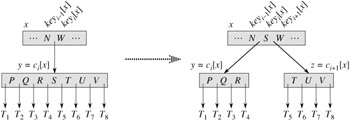
Figure 18.5: Splitting a node with t = 4. Node y is split into two nodes, y and z, and the median key S of y is moved up into y's parent.

B-TREE-SPLIT-CHILD(x, i, y)
 1  z ← ALLOCATE-NODE()
 2  leaf[z] ← leaf[y]
 3  n[z] ← t - 1
 4  for j ← 1 to t - 1
 5       do key_j[z] ← key_j+t[y]
 6  if not leaf [y]
 7     then for j ← 1 to t
 8              do c_j[z] ← c_j+t[y]
 9  n[y] ← t - 1
10  for j ← n[x] + 1 downto i + 1
11       do c_j+1[x] ← c_j [x]
12  c_i+1[x] ← z
13  for j ← n[x] downto i
14       do key_j+1[x] ← key_j[x]
15  key_i[x] ← key_t[y]
16  n[x] ← n[x] + 1
17  DISK-WRITE(y)
18  DISK-WRITE(z)
19  DISK-WRITE(x)

B-TREE-SPLIT-CHILD works by straightforward "cutting and pasting." Here, y is the ith child of x and is the node being split. Node y originally has 2t children (2t - 1 keys) but is reduced to t children (t - 1 keys) by this operation. Node z "adopts" the t largest children (t - 1 keys) of y, and z becomes a new child of x, positioned just after y in x's table of children. The median key of y moves up to become the key in x that separates y and z.

Lines 1-8 create node z and give it the larger t - 1 keys and corresponding t children of y. Line 9 adjusts the key count for y. Finally, lines 10-16 insert z as a child of x, move the median key from y up to x in order to separate y from z, and adjust x's key count. Lines 17-19 write out all modified disk pages. The CPU time used by B-TREE-SPLIT-CHILD is Θ(t), due to the loops on lines 4-5 and 7-8. (The other loops run for O(t) iterations.) The procedure performs O(1) disk operations.

Inserting a key into a B-tree in a single pass down the tree

We insert a key k into a B-tree T of height h in a single pass down the tree, requiring O(h) disk accesses. The CPU time required is O(th) = O(t log_t n). The B-TREE-INSERT procedure uses B-TREE-SPLIT-CHILD to guarantee that the recursion never descends to a full node.

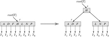
B-TREE-INSERT(T, k)
 1  r ← root[T]
 2  if n[r] = 2t - 1
 3     then s ← ALLOCATE-NODE()
 4         root[T] ← s
 5         leaf[s] ← FALSE
 6         n[s] ← 0
 7         c₁[s] ← r
 8         B-TREE-SPLIT-CHILD(s, 1, r)
 9         B-TREE-INSERT-NONFULL(s, k)
10    else B-TREE-INSERT-NONFULL(r, k)

Lines 3-9 handle the case in which the root node r is full: the root is split and a new node s (having two children) becomes the root. Splitting the root is the only way to increase the height of a B-tree. Figure 18.6 illustrates this case. Unlike a binary search tree, a B-tree increases in height at the top instead of at the bottom. The procedure finishes by calling B-TREE-INSERT-NONFULL to perform the insertion of key k in the tree rooted at the nonfull root node. B-TREE-INSERT-NONFULL recurses as necessary down the tree, at all times guaranteeing that the node to which it recurses is not full by calling B-TREE-SPLIT-CHILD as necessary.

Figure 18.6: Splitting the root with t = 4. Root node r is split in two, and a new root node s is created. The new root contains the median key of r and has the two halves of r as children. The B-tree grows in height by one when the root is split.

The auxiliary recursive procedure B-TREE-INSERT-NONFULL inserts key k into node x, which is assumed to be nonfull when the procedure is called. The operation of B-TREE-INSERT and the recursive operation of B-TREE-INSERT-NONFULL guarantee that this assumption is true.

B-TREE-INSERT-NONFULL(x, k)
 1  i ← n[x]
 2  if leaf[x]
 3     then while i ≥ 1 and k < key_i[x]
 4            do key_i+1[x] ← key_i[x]
 5                   i ← i - 1
 6             key_i+1[x] ← k
 7             n[x] ← n[x] + 1
 8             DISK-WRITE(x)
 9     else while i ≥ 1 and k < key_i[x]
10             do i ← i - 1
11           i ← i + 1
12           DISK-READ(c_i[x])
13           if n[c_i[x]] = 2t - 1
14             then B-TREE-SPLIT-CHILD(x, i, c_i[x])
15                    if k> key_i[x]
16                      then i ← i + 1
17           B-TREE-INSERT-NONFULL(c_i[x], k)

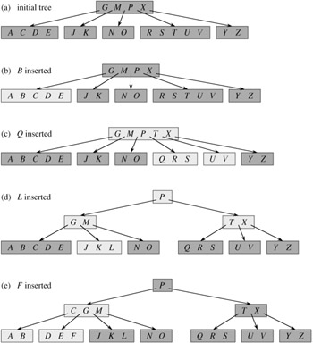
The B-TREE-INSERT-NONFULL procedure works as follows. Lines 3-8 handle the case in which x is a leaf node by inserting key k into x. If x is not a leaf node, then we must insert k into the appropriate leaf node in the subtree rooted at internal node x. In this case, lines 9-11 determine the child of x to which the recursion descends. Line 13 detects whether the recursion would descend to a full child, in which case line 14 uses B-TREE-SPLIT-CHILD to split that child into two nonfull children, and lines 15-16 determine which of the two children is now the correct one to descend to. (Note that there is no need for a DISK-READ(c_i [x]) after line 16 increments i, since the recursion will descend in this case to a child that was just created by B-TREE-SPLIT-CHILD.) The net effect of lines 13-16 is thus to guarantee that the procedure never recurses to a full node. Line 17 then recurses to insert k into the appropriate subtree. Figure 18.7 illustrates the various cases of inserting into a B-tree.

Figure 18.7: Inserting keys into a B-tree. The minimum degree t for this B-tree is 3, so a node can hold at most 5 keys. Nodes that are modified by the insertion process are lightly shaded. (a) The initial tree for this example. (b) The result of inserting B into the initial tree; this is a simple insertion into a leaf node. (c) The result of inserting Q into the previous tree. The node RSTUV is split into two nodes containing RS and UV, the key T is moved up to the root, and Q is inserted in the leftmost of the two halves (the RS node). (d) The result of inserting L into the previous tree. The root is split right away, since it is full, and the B-tree grows in height by one. Then L is inserted into the leaf containing JK. (e) The result of inserting F into the previous tree. The node ABCDE is split before F is inserted into the rightmost of the two halves (the DE node).

The number of disk accesses performed by B-TREE-INSERT is O(h) for a B-tree of height h, since only O(1) DISK-READ and DISK-WRITE operations are performed between calls to B-TREE-INSERT-NONFULL. The total CPU time used is O(th) = O(t log_t n). Since B-TREE-INSERT-NONFULL is tail-recursive, it can be alternatively implemented as a while loop, demonstrating that the number of pages that need to be in main memory at any time is O(1).

Exercises 18.2-1

Show the results of inserting the keys

F, S, Q, K, C, L, H, T, V, W, M, R, N, P, A, B, X, Y, D, Z, E

in order into an empty B-tree with minimum degree 2. Only draw the configurations of the tree just before some node must split, and also draw the final configuration.

Exercises 18.2-2

Explain under what circumstances, if any, redundant DISK-READ or DISK-WRITE operations are performed during the course of executing a call to B-TREE-INSERT. (A redundant DISK-READ is a DISK-READ for a page that is already in memory. A redundant DISK-WRITE writes to disk a page of information that is identical to what is already stored there.)

Exercises 18.2-3

Explain how to find the minimum key stored in a B-tree and how to find the predecessor of a given key stored in a B-tree.

Exercises 18.2-4: ⋆

Suppose that the keys {1, 2, ..., n} are inserted into an empty B-tree with minimum degree 2. How many nodes does the final B-tree have?

Exercises 18.2-5

Since leaf nodes require no pointers to children, they could conceivably use a different (larger) t value than internal nodes for the same disk page size. Show how to modify the procedures for creating and inserting into a B-tree to handle this variation.

Exercises 18.2-6

Suppose that B-TREE-SEARCH is implemented to use binary search rather than linear search within each node. Show that this change makes the CPU time required O(lg n), independently of how t might be chosen as a function of n.

Exercises 18.2-7

Suppose that disk hardware allows us to choose the size of a disk page arbitrarily, but that the time it takes to read the disk page is a + bt, where a and b are specified constants and t is the minimum degree for a B-tree using pages of the selected size. Describe how to choose t so as to minimize (approximately) the B-tree search time. Suggest an optimal value of t for the case in which a = 5 milliseconds and b = 10 microseconds.