|
|
< Day Day Up > |
|
The strategy followed by depth-first search is, as its name implies, to search "deeper" in the graph whenever possible. In depth-first search, edges are explored out of the most recently discovered vertex v that still has unexplored edges leaving it. When all of v's edges have been explored, the search "backtracks" to explore edges leaving the vertex from which v was discovered. This process continues until we have discovered all the vertices that are reachable from the original source vertex. If any undiscovered vertices remain, then one of them is selected as a new source and the search is repeated from that source. This entire process is repeated until all vertices are discovered.
As in breadth-first search, whenever a vertex v is discovered during a scan of the adjacency list of an already discovered vertex u, depth-first search records this event by setting v's predecessor field π[v] to u. Unlike breadth-first search, whose predecessor subgraph forms a tree, the predecessor subgraph produced by a depth-first search may be composed of several trees, because the search may be repeated from multiple sources.[2] The predecessor subgraph of a depth-first search is therefore defined slightly differently from that of a breadth-first search: we let Gπ = (V, Eπ), where
Eπ = {(π[v], v) : v ∈ V and π[v] ≠ NIL}.
The predecessor subgraph of a depth-first search forms a depth-first forest composed of several depth-first trees. The edges in Eπ are called tree edges.
As in breadth-first search, vertices are colored during the search to indicate their state. Each vertex is initially white, is grayed when it is discovered in the search, and is blackened when it is finished, that is, when its adjacency list has been examined completely. This technique guarantees that each vertex ends up in exactly one depth-first tree, so that these trees are disjoint.
Besides creating a depth-first forest, depth-first search also timestamps each vertex. Each vertex v has two timestamps: the first timestamp d[v] records when v is first discovered (and grayed), and the second timestamp f [v] records when the search finishes examining v's adjacency list (and blackens v). These timestamps are used in many graph algorithms and are generally helpful in reasoning about the behavior of depth-first search.
The procedure DFS below records when it discovers vertex u in the variable d[u] and when it finishes vertex u in the variable f [u]. These timestamps are integers between 1 and 2 |V|, since there is one discovery event and one finishing event for each of the |V| vertices. For every vertex u,
Vertex u is WHITE before time d[u], GRAY between time d[u] and time f [u], and BLACK thereafter.
The following pseudocode is the basic depth-first-search algorithm. The input graph G may be undirected or directed. The variable time is a global variable that we use for timestamping.
DFS(G)
1  for each vertex u ∈ V [G]
2       do color[u] ← WHITE
3          π[u] ← NIL
4  time ← 0
5  for each vertex u ∈ V [G]
6       do if color[u] = WHITE
7             then DFS-VISIT(u)
DFS-VISIT(u)
1  color[u] ← GRAY     ▹White vertex u has just been discovered.
2  time ← time +1
3  d[u] time
4  for each v ∈ Adj[u]  ▹Explore edge(u, v).
5       do if color[v] = WHITE
6             then π[v] ← u
7                         DFS-VISIT(v)
8  color[u] BLACK      ▹ Blacken u; it is finished.
9  f [u] ▹ time ← time +1
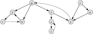
Figure 22.4 illustrates the progress of DFS on the graph shown in Figure 22.2.
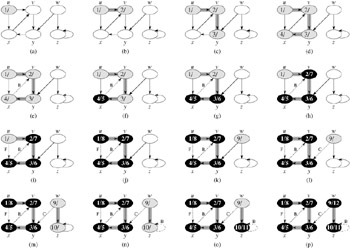
Procedure DFS works as follows. Lines 1-3 paint all vertices white and initialize their π fields to NIL. Line 4 resets the global time counter. Lines 5-7 check each vertex in V in turn and, when a white vertex is found, visit it using DFS-VISIT. Every time DFS-VISIT(u) is called in line 7, vertex u becomes the root of a new tree in the depth-first forest. When DFS returns, every vertex u has been assigned a discovery time d[u] and a finishing time f [u].
In each call DFS-VISIT(u), vertex u is initially white. Line 1 paints u gray, line 2 increments the global variable time, and line 3 records the new value of time as the discovery time d[u]. Lines 4-7 examine each vertex v adjacent to u and recursively visit v if it is white. As each vertex v ∈ Adj[u] is considered in line 4, we say that edge (u, v) is explored by the depth-first search. Finally, after every edge leaving u has been explored, lines 8-9 paint u black and record the finishing time in f [u].
Note that the results of depth-first search may depend upon the order in which the vertices are examined in line 5 of DFS, and upon the order in which the neighbors of a vertex are visited in line 4 of DFS-VISIT. These different visitation orders tend not to cause problems in practice, as any depth-first search result can usually be used effectively, with essentially equivalent results.
What is the running time of DFS? The loops on lines 1-3 and lines 5-7 of DFS take time Θ(V), exclusive of the time to execute the calls to DFS-VISIT. As we did for breadth-first search, we use aggregate analysis. The procedure DFS-VISIT is called exactly once for each vertex v ∈ V , since DFS-VISIT is invoked only on white vertices and the first thing it does is paint the vertex gray. During an execution of DFS-VISIT(v), the loop on lines 4-7 is executed |Adj[v]| times. Since
the total cost of executing lines 4-7 of DFS-VISIT is Θ(E). The running time of DFS is therefore Θ(V + E).
Depth-first search yields valuable information about the structure of a graph. Perhaps the most basic property of depth-first search is that the predecessor subgraph Gπ does indeed form a forest of trees, since the structure of the depth-first trees exactly mirrors the structure of recursive calls of DFS-VISIT. That is, u = π[v] if and only if DFS-VISIT(v) was called during a search of u's adjacency list. Additionally, vertex v is a descendant of vertex u in the depth-first forest if and only if v is discovered during the time in which u is gray.
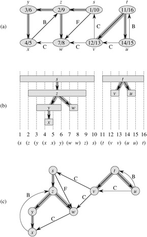
Another important property of depth-first search is that discovery and finishing times have parenthesis structure. If we represent the discovery of vertex u with a left parenthesis "(u" and represent its finishing by a right parenthesis "u)", then the history of discoveries and finishings makes a well-formed expression in the sense that the parentheses are properly nested. For example, the depth-first search of Figure 22.5(a) corresponds to the parenthesization shown in Figure 22.5(b). Another way of stating the condition of parenthesis structure is given in the following theorem.
In any depth-first search of a (directed or undirected) graph G = (V, E), for any two vertices u and v, exactly one of the following three conditions holds:
the intervals [d[u], f[u]] and [d[v], f[v]] are entirely disjoint, and neither u nor v is a descendant of the other in the depth-first forest,
the interval [d[u], f[u]] is contained entirely within the interval [d[v], f[v]], and u is a descendant of v in a depth-first tree, or
the interval [d[v], f[v]] is contained entirely within the interval [d[u], f[u]], and v is a descendant of u in a depth-first tree.
Proof We begin with the case in which d[u] < d[v]. There are two subcases to consider, according to whether d[v] < f[u] or not. The first subcase occurs when d[v] < f[u], so v was discovered while u was still gray. This implies that v is a descendant of u. Moreover, since v was discovered more recently than u, all of its outgoing edges are explored, and v is finished, before the search returns to and finishes u. In this case, therefore, the interval [d[v], f[v]] is entirely contained within the interval [d[u], f[u]]. In the other subcase, f[u] < d[v], and inequality (22.2) implies that the intervals [d[u], f[u]] and [d[v], f[v]] are disjoint. Because the intervals are disjoint, neither vertex was discovered while the other was gray, and so neither vertex is a descendant of the other.
The case in which d[v] < d[u] is similar, with the roles of u and v reversed in the above argument.
Vertex v is a proper descendant of vertex u in the depth-first forest for a (directed or undirected) graph G if and only if d[u] < d[v] < f[v] < f[u].
Proof Immediate from Theorem 22.7.
The next theorem gives another important characterization of when one vertex is a descendant of another in the depth-first forest.
In a depth-first forest of a (directed or undirected) graph G = (V, E), vertex v is a descendant of vertex u if and only if at the time d[u] that the search discovers u, vertex v can be reached from u along a path consisting entirely of white vertices.
Proof →: Assume that v is a descendant of u. Let w be any vertex on the path between u and v in the depth-first tree, so that w is a descendant of u. By Corollary 22.8, d[u] < d[w], and so w is white at time d[u].
←: Suppose that vertex v is reachable from u along a path of white vertices at time d[u], but v does not become a descendant of u in the depth-first tree. Without loss of generality, assume that every other vertex along the path becomes a descendant of u. (Otherwise, let v be the closest vertex to u along the path that doesn't become a descendant of u.) Let w be the predecessor of v in the path, so that w is a descendant of u (w and u may in fact be the same vertex) and, by Corollary 22.8, f[w] ≤ f[u]. Note that v must be discovered after u is discovered, but before w is finished. Therefore, d[u] < d[v] < f[w] ≤ f[u]. Theorem 22.7 then implies that the interval [d[v], f[v]] is contained entirely within the interval [d[u], f[u]]. By Corollary 22.8, v must after all be a descendant of u.
Another interesting property of depth-first search is that the search can be used to classify the edges of the input graph G = (V, E). This edge classification can be used to glean important information about a graph. For example, in the next section, we shall see that a directed graph is acyclic if and only if a depth-first search yields no "back" edges (Lemma 22.11).
We can define four edge types in terms of the depth-first forest Gπ produced by a depth-first search on G.
Tree edges are edges in the depth-first forest Gπ. Edge (u, v) is a tree edge if v was first discovered by exploring edge (u, v).
Back edges are those edges (u, v) connecting a vertex u to an ancestor v in a depth-first tree. Self-loops, which may occur in directed graphs, are considered to be back edges.
Forward edges are those nontree edges (u, v) connecting a vertex u to a descendant v in a depth-first tree.
Cross edges are all other edges. They can go between vertices in the same depth-first tree, as long as one vertex is not an ancestor of the other, or they can go between vertices in different depth-first trees.
In Figures 22.4 and 22.5, edges are labeled to indicate their type. Figure 22.5(c) also shows how the graph of Figure 22.5(a) can be redrawn so that all tree and forward edges head downward in a depth-first tree and all back edges go up. Any graph can be redrawn in this fashion.
The DFS algorithm can be modified to classify edges as it encounters them. The key idea is that each edge (u, v) can be classified by the color of the vertex v that is reached when the edge is first explored (except that forward and cross edges are not distinguished):
WHITE indicates a tree edge,
GRAY indicates a back edge, and
BLACK indicates a forward or cross edge.
The first case is immediate from the specification of the algorithm. For the second case, observe that the gray vertices always form a linear chain of descendants corresponding to the stack of active DFS-VISIT invocations; the number of gray vertices is one more than the depth in the depth-first forest of the vertex most recently discovered. Exploration always proceeds from the deepest gray vertex, so an edge that reaches another gray vertex reaches an ancestor. The third case handles the remaining possibility; it can be shown that such an edge (u, v) is a forward edge if d[u] < d[v] and a cross edge if d[u] > d[v]. (See Exercise 22.3-4.)
In an undirected graph, there may be some ambiguity in the type classification, since (u, v) and (v, u) are really the same edge. In such a case, the edge is classified as the first type in the classification list that applies. Equivalently (see Exercise 22.3-5), the edge is classified according to whichever of (u, v) or (v, u) is encountered first during the execution of the algorithm.
We now show that forward and cross edges never occur in a depth-first search of an undirected graph.
In a depth-first search of an undirected graph G, every edge of G is either a tree edge or a back edge.
Proof Let (u, v) be an arbitrary edge of G, and suppose without loss of generality that d[u] < d[v]. Then, v must be discovered and finished before we finish u (while u is gray), since v is on u's adjacency list. If the edge (u, v) is explored first in the direction from u to v, then v is undiscovered (white) until that time, for otherwise we would have explored this edge already in the direction from v to u. Thus, (u, v) becomes a tree edge. If (u, v) is explored first in the direction from v to u, then (u, v) is a back edge, since u is still gray at the time the edge is first explored.
We shall see several applications of these theorems in the following sections.
Make a 3-by-3 chart with row and column labels WHITE, GRAY, and BLACK. In each cell (i, j), indicate whether, at any point during a depth-first search of a directed graph, there can be an edge from a vertex of color i to a vertex of color j. For each possible edge, indicate what edge types it can be. Make a second such chart for depth-first search of an undirected graph.
Show how depth-first search works on the graph of Figure 22.6. Assume that the for loop of lines 5-7 of the DFS procedure considers the vertices in alphabetical order, and assume that each adjacency list is ordered alphabetically. Show the discovery and finishing times for each vertex, and show the classification of each edge.
Show that edge (u, v) is
a tree edge or forward edge if and only if d[u] < d[v] < f[v] < f[u],
a back edge if and only if d[v] < d[u] < f[u] < f[v], and
a cross edge if and only if d[v] < f[v] < d[u] < f[u].
Show that in an undirected graph, classifying an edge (u, v) as a tree edge or a back edge according to whether (u, v) or (v, u) is encountered first during the depth-first search is equivalent to classifying it according to the priority of types in the classification scheme.
Give a counterexample to the conjecture that if there is a path from u to v in a directed graph G, and if d[u] < d[v] in a depth-first search of G, then v is a descendant of u in the depth-first forest produced.
Give a counterexample to the conjecture that if there is a path from u to v in a directed graph G, then any depth-first search must result in d[v] ≤ f[u].
Modify the pseudocode for depth-first search so that it prints out every edge in the directed graph G, together with its type. Show what modifications, if any, must be made if G is undirected.
Explain how a vertex u of a directed graph can end up in a depth-first tree containing only u, even though u has both incoming and outgoing edges in G.
Show that a depth-first search of an undirected graph G can be used to identify the connected components of G, and that the depth-first forest contains as many trees as G has connected components. More precisely, show how to modify depth-first search so that each vertex v is assigned an integer label cc[v] between 1 and k, where k is the number of connected components of G, such that cc[u] = cc[v] if and only if u and v are in the same connected component.
[2]It may seem arbitrary that breadth-first search is limited to only one source whereas depth-first search may search from multiple sources. Although conceptually, breadth-first search could proceed from multiple sources and depth-first search could be limited to one source, our approach reflects how the results of these searches are typically used. Breadth-first search is usually employed to find shortest-path distances (and the associated predecessor subgraph) from a given source. Depth-first search is often a subroutine in another algorithm, as we shall see later in this chapter.
|
|
< Day Day Up > |
|