|
|
< Day Day Up > |
|
In this section, we give a graph-theoretic definition of flow networks, discuss their properties, and define the maximum-flow problem precisely. We also introduce some helpful notation.
A flow network G = (V, E) is a directed graph in which each edge (u, v) ∈E has a nonnegative capacity c(u, v) ≥ 0. If (u, v) ∉ E, we assume that c(u, v) = 0. We distinguish two vertices in a flow network: a source s and a sink t. For convenience, we assume that every vertex lies on some path from the source to the sink. That is, for every vertex v ∈ V, there is a path ![]() The graph is therefore connected, and |E| ≥ |V | - 1. Figure 26.1 shows an example of a flow network.
The graph is therefore connected, and |E| ≥ |V | - 1. Figure 26.1 shows an example of a flow network.
We are now ready to define flows more formally. Let G = (V, E) be a flow network with a capacity function c. Let s be the source of the network, and let t be the sink. A flow in G is a real-valued function f : V × V → R that satisfies the following three properties:
Capacity constraint: For all u, v ∈ V, we require f (u, v) ≤ c(u, v).
Skew symmetry: For all u, v ∈ V, we require f (u, v) = - f (v, u).
Flow conservation: For all u ∈ V - {s, t}, we require
The quantity f (u, v), which can be positive, zero, or negative, is called the flow from vertex u to vertex v. The value of a flow f is defined as
| (26.1) |
that is, the total flow out of the source. (Here, the |·| notation denotes flow value, not absolute value or cardinality.) In the maximum-flow problem, we are given a flow network G with source s and sink t, and we wish to find a flow of maximum value.
Before seeing an example of a network-flow problem, let us briefly explore the three flow properties. The capacity constraint simply says that the flow from one vertex to another must not exceed the given capacity. Skew symmetry is a notational convenience that says that the flow from a vertex u to a vertex v is the negative of the flow in the reverse direction. The flow-conservation property says that the total flow out of a vertex other than the source or sink is 0. By skew symmetry, we can rewrite the flow-conservation property as
for all v ∈ V - {s, t}. That is, the total flow into a vertex is 0.
When neither (u, v) nor (v, u) is in E, there can be no flow between u and v, and f(u, v) = f(v, u) = 0. (Exercise 26.1-1 asks you to prove this property formally.)
Our last observation concerning the flow properties deals with flows that are positive. The total positive flow entering a vertex v is defined by
| (26.2) |
The total positive flow leaving a vertex is defined symmetrically. We define the total net flow at a vertex to be the total positive flow leaving a vertex minus the total positive flow entering a vertex. One interpretation of the flow-conservation property is that the total positive flow entering a vertex other than the source or sink must equal the total positive flow leaving that vertex. This property, that the total net flow at a vertex must equal 0, is often informally referred to as "flow in equals flow out."
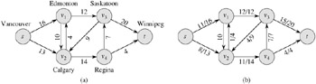
A flow network can model the trucking problem shown in Figure 26.1(a). The Lucky Puck Company has a factory (source s) in Vancouver that manufactures hockey pucks, and it has a warehouse (sink t) in Winnipeg that stocks them. Lucky Puck leases space on trucks from another firm to ship the pucks from the factory to the warehouse. Because the trucks travel over specified routes (edges) between cities (vertices) and have a limited capacity, Lucky Puck can ship at most c(u, v) crates per day between each pair of cities u and v in Figure 26.1(a). Lucky Puck has no control over these routes and capacities and so cannot alter the flow network shown in Figure 26.1(a). Their goal is to determine the largest number p of crates per day that can be shipped and then to produce this amount, since there is no point in producing more pucks than they can ship to their warehouse. Lucky Puck is not concerned with how long it takes for a given puck to get from the factory to the warehouse; they care only that p crates per day leave the factory and p crates per day arrive at the warehouse.
On the surface, it seems appropriate to model the "flow" of shipments with a flow in this network because the number of crates shipped per day from one city to another is subject to a capacity constraint. Additionally, flow conservation must be obeyed, for in a steady state, the rate at which pucks enter an intermediate city must equal the rate at which they leave. Otherwise, crates would accumulate at intermediate cities.
There is one subtle difference between shipments and flows, however. Lucky Puck may ship pucks from Edmonton to Calgary, and they may also ship pucks from Calgary to Edmonton. Suppose that they ship 8 crates per day from Edmonton (v1 in Figure 26.1) to Calgary (v2) and 3 crates per day from Calgary to Edmonton. It may seem natural to represent these shipments directly by flows, but we cannot. The skew-symmetry constraint requires that f (v1, v2) = - f (v2, v1), but this is clearly not the case if we consider f(v1, v2) = 8 and f(v2, v1) = 3.
Lucky Puck may realize that it is pointless to ship 8 crates per day from Edmonton to Calgary and 3 crates from Calgary to Edmonton, when they could achieve the same net effect by shipping 5 crates from Edmonton to Calgary and 0 crates from Calgary to Edmonton (and presumably use fewer resources in the process). We represent this latter scenario with a flow: we have f (v1, v2) = 5 and f(v2, v1) = -5. In effect, 3 of the 8 crates per day from v1 to v2 are canceled by 3 crates per day from v2 to v1.
In general, cancellation allows us to represent the shipments between two cities by a flow that is positive along at most one of the two edges between the corresponding vertices. That is, any situation in which pucks are shipped in both directions between two cities can be transformed using cancellation into an equivalent situation in which pucks are shipped in one direction only: the direction of positive flow.
Given a flow f that arose from, say, physical shipments, we cannot reconstruct the exact shipments. If we know that f(u, v) = 5, this flow may be because 5 units were shipped from u to v, or it may be because 8 units were shipped from u to v and 3 units were shipped from v to u. Typically, we shall not care how the actual physical shipments are set up; for any pair of vertices, we care only about the net amount that travels between them. If we do care about the underlying shipments, then we should be using a different model, one that retains information about shipments in both directions.
Cancellation will arise implicitly in the algorithms in this chapter. Suppose that edge (u, v) has a flow value of f(u, v). In the course of an algorithm, we may increase the flow on edge (v, u) by some amount d. Mathematically, this operation must decrease f(u, v) by d and, conceptually, we can think of these d units as canceling d units of flow that are already on edge (u, v).
A maximum-flow problem may have several sources and sinks, rather than just one of each. The Lucky Puck Company, for example, might actually have a set of m factories {s1, s2, . . . , sm} and a set of n warehouses {t1, t2, . . . , tn}, as shown in Figure 26.2(a). Fortunately, this problem is no harder than ordinary maximum flow.
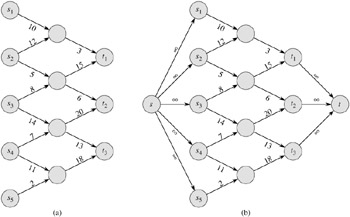
We can reduce the problem of determining a maximum flow in a network with multiple sources and multiple sinks to an ordinary maximum-flow problem. Figure 26.2(b) shows how the network from (a) can be converted to an ordinary flow network with only a single source and a single sink. We add a supersource s and add a directed edge (s, si) with capacity c(s, si) = ∞ for each i = 1, 2, . . . , m. We also create a new supersink t and add a directed edge (ti, t) with capacity c(ti, t) = ∞ for each i = 1, 2, . . . , n. Intuitively, any flow in the network in (a) corresponds to a flow in the network in (b), and vice versa. The single source s simply provides as much flow as desired for the multiple sources si, and the single sink t likewise consumes as much flow as desired for the multiple sinks ti. Exercise 26.1-3 asks you to prove formally that the two problems are equivalent.
We shall be dealing with several functions (like f) that take as arguments two vertices in a flow network. In this chapter, we shall use an implicit summation notation in which either argument, or both, may be a set of vertices, with the interpretation that the value denoted is the sum of all possible ways of replacing the arguments with their members. For example, if X and Y are sets of vertices, then
Thus, the flow-conservation constraint can be expressed as the condition that f(u, V) = 0 for all u ∈ V - {s, t}. Also, for convenience, we shall typically omit set braces when they would otherwise be used in the implicit summation notation. For example, in the equation f (s, V - s) = f(s, V), the term V - s means the set V - {s}.
The implicit set notation often simplifies equations involving flows. The following lemma, whose proof is left as Exercise 26.1-4, captures several of the most commonly occurring identities that involve flows and the implicit set notation.
Let G = (V, E) be a flow network, and let f be a flow in G. Then the following equalities hold:
For all X ⊆ V, we have f(X, X) = 0.
For all X, Y ⊆ V, we have f(X, Y) = - f (Y, X).
For all X, Y, Z ⊆ V with X ∩ Y = Ø, we have the sums f(X ∪ Y, Z) =
f(X, Z) + f(Y, Z) and f(Z, X ∪ Y) = f (Z, X) + f(Z, Y).
As an example of working with the implicit summation notation, we can prove that the value of a flow is the total flow into the sink; that is,
Intuitively, we expect this property to hold. By flow conservation, all vertices other than the source and sink have equal amounts of total positive flow entering and leaving. The source has, by definition, a total net flow that is greater than 0; that is, more positive flow leaves the source than enters it. Symmetrically, the sink is the only vertex that can have a total net flow that is less than 0; that is, more positive flow enters the sink than leaves it. Our formal proof goes as follows:
|
|f| |
= |
f(s, V) |
(by definition) |
|
= |
f(V, V) - f (V - s, V) |
(by Lemma 26.1, part (3)) |
|
|
= |
- f(V - s, V) |
(by Lemma 26.1, part (1)) |
|
|
= |
f(V, V - s) |
(by Lemma 26.1, part (2)) |
|
|
= |
f(V, t) + f(V, V - s - t) |
(by Lemma 26.1, part (3)) |
|
|
= |
f(V, t) |
(by flow conservation). |
Later in this chapter, we shall generalize this result (Lemma 26.5).
Using the definition of a flow, prove that if (u, v) ∉ E and (v, u) ∉ E then f(u, v) = f(v, u) = 0.
Prove that for any vertex v other than the source or sink, the total positive flow entering v must equal the total positive flow leaving v.
Extend the flow properties and definitions to the multiple-source, multiple-sink problem. Show that any flow in a multiple-source, multiple-sink flow network corresponds to a flow of identical value in the single-source, single-sink network obtained by adding a supersource and a supersink, and vice versa.
For the flow network G = (V, E) and flow f shown in Figure 26.1(b), find a pair of subsets X, Y ⊆ V for which f(X, Y) = - f(V - X, Y). Then, find a pair of subsets X, Y ⊆ V for which f (X, Y) ≠ - f(V - X, Y).
Let f be a flow in a network, and let α be a real number. The scalar flow product, denoted α f, is a function from V × V to R defined by
(αf)(u, v) = α · f (u, v).
Prove that the flows in a network form a convex set. That is, show that if f1 and f2 are flows, then so is αf1 + (1 - α) f2 for all α in the range 0 ≤ α ≤ 1.
Professor Adam has two children who, unfortunately, dislike each other. The problem is so severe that not only do they refuse to walk to school together, but in fact each one refuses to walk on any block that the other child has stepped on that day. The children have no problem with their paths crossing at a corner. Fortunately both the professor's house and the school are on corners, but beyond that he is not sure if it is going to be possible to send both of his children to the same school. The professor has a map of his town. Show how to formulate the problem of determining if both his children can go to the same school as a maximum-flow problem.
|
|
< Day Day Up > |
|