Decision problems vs. optimization problems

Many problems of interest are optimization problems, in which each feasible (i.e., "legal") solution has an associated value, and we wish to find the feasible solution with the best value. For example, in a problem that we call SHORTEST-PATH, we are given an undirected graph G and vertices u and v, and we wish to find the path from u to v that uses the fewest edges. (In other words, SHORTEST-PATH is the single-pair shortest-path problem in an unweighted, undirected graph.) NP-completeness applies directly not to optimization problems, however, but to decision problems, in which the answer is simply "yes" or "no" (or, more formally, "1" or "0").

Although showing that a problem is NP-complete confines us to the realm of decision problems, there is a convenient relationship between optimization problems and decision problems. We usually can cast a given optimization problem as a related decision problem by imposing a bound on the value to be optimized. For SHORTEST-PATH, for example, a related decision problem, which we call PATH, is whether, given a directed graph G, vertices u and v, and an integer k, a path exists from u to v consisting of at most k edges.

The relationship between an optimization problem and its related decision problem works in our favor when we try to show that the optimization problem is "hard." That is because the decision problem is in a sense "easier," or at least "no harder." As a specific example, we can solve PATH by solving SHORTEST-PATH and then comparing the number of edges in the shortest path found to the value of the decision-problem parameter k. In other words, if an optimization problem is easy, its related decision problem is easy as well. Stated in a way that has more relevance to NP-completeness, if we can provide evidence that a decision problem is hard, we also provide evidence that its related optimization problem is hard. Thus, even though it restricts attention to decision problems, the theory of NP-completeness often has implications for optimization problems as well.

Reductions

The above notion of showing that one problem is no harder or no easier than another applies even when both problems are decision problems. We take advantage of this idea in almost every NP-completeness proof, as follows. Let us consider a decision problem, say A, which we would like to solve in polynomial time. We call the input to a particular problem an instance of that problem; for example, in PATH, an instance would be a particular graph G, particular vertices u and v of G, and a particular integer k. Now suppose that there is a different decision problem, say B, that we already know how to solve in polynomial time. Finally, suppose that we have a procedure that transforms any instance α of A into some instance β of B with the following characteristics:

The transformation takes polynomial time.
The answers are the same. That is, the answer for α is "yes" if and only if the answer for β is also "yes."

We call such a procedure a polynomial-time reduction algorithm and, as Figure 34.1 shows, it provides us a way to solve problem A in polynomial time:

Given an instance α of problem A, use a polynomial-time reduction algorithm to transform it to an instance β of problem B.
Run the polynomial-time decision algorithm for B on the instance β.
Use the answer for β as the answer for α.

Figure 34.1: Using a polynomial-time reduction algorithm to solve a decision problem A in polynomial time, given a polynomial-time decision algorithm for another problem B. In polynomial time, we transform an instance α of A into an instance β of B, we solve B in polynomial time, and we use the answer for β as the answer for α.

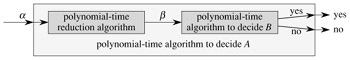
As long as each of these steps takes polynomial time, all three together do also, and so we have a way to decide on α in polynomial time. In other words, by "reducing" solving problem A to solving problem B, we use the "easiness" of B to prove the "easiness" of A.

Recalling that NP-completeness is about showing how hard a problem is rather than how easy it is, we use polynomial-time reductions in the opposite way to show that a problem is NP-complete. Let us take the idea a step further, and show how we could use polynomial-time reductions to show that no polynomial-time algorithm can exist for a particular problem B. Suppose we have a decision problem A for which we already know that no polynomial-time algorithm can exist. (Let us not concern ourselves for now with how to find such a problem A.) Suppose further that we have a polynomial-time reduction transforming instances of A to instances of B. Now we can use a simple proof by contradiction to show that no polynomial-time algorithm can exist for B. Suppose otherwise, i.e., suppose that B has a polynomial-time algorithm. Then, using the method shown in Figure 34.1, we would have a way to solve problem A in polynomial time, which contradicts our assumption that there is no polynomial-time algorithm for A.

For NP-completeness, we cannot assume that there is absolutely no polynomial-time algorithm for problem A. The proof methodology is similar, however, in that we prove that problem B is NP-complete on the assumption that problem A is also NP-complete.

A first NP-complete problem

Because the technique of reduction relies on having a problem already known to be NP-complete in order to prove a different problem NP-complete, we need a "first" NP-complete problem. The problem we shall use is the circuit-satisfiability problem, in which we are given a boolean combinational circuit composed of AND, OR, and NOT gates, and we wish to know whether there is any set of boolean inputs to this circuit that causes its output to be 1. We shall prove that this first problem is NP-complete in Section 34.3.