List of Figures

Chapter 2: Getting Started

Figure 2.1: Sorting a hand of cards using insertion sort.
Figure 2.2: The operation of INSERTION-SORT on the array A = 〈5, 2, 4, 6, 1, 3〉. Array indices appear above the rectangles, and values stored in the array positions appear within the rectangles. (a)–(e) The iterations of the for loop of lines 1–8. In each iteration, the black rectangle holds the key taken from A[j], which is compared with the values in shaded rectangles to its left in the test of line 5. Shaded arrows show array values moved one position to the right in line 6, and black arrows indicate where the key is moved to in line 8. (f) The final sorted array.
Figure 2.3: The operation of lines 10–17 in the call MERGE(A, 9, 12, 16), when the subarray A[9 ‥ 16] contains the sequence 〈2, 4, 5, 7, 1, 2, 3, 6〉. After copying and inserting sentinels, the array L contains 〈2, 4, 5, 7, ∞〉, and the array R contains 〈1, 2, 3, 6, ∞〉. Lightly shaded positions in A contain their final values, and lightly shaded positions in L and R contain values that have yet to be copied back into A. Taken together, the lightly shaded positions always comprise the values originally in A[9 ‥ 16], along with the two sentinels. Heavily shaded positions in A contain values that will be copied over, and heavily shaded positions in L and R contain values that have already been copied back into A. (a)–(h) The arrays A, L, and R, and their respective indices k, i, and j prior to each iteration of the loop of lines 12–17. (i) The arrays and indices at termination. At this point, the subarray in A[9 ‥ 16] is sorted, and the two sentinels in L and R are the only two elements in these arrays that have not been copied into A.
Figure 2.4: The operation of merge sort on the array A = 〈5, 2, 4, 7, 1, 3, 2, 6〉. The lengths of the sorted sequences being merged increase as the algorithm progresses from bottom to top.
Figure 2.5: The construction of a recursion tree for the recurrence T(n) = 2T(n/2) + cn. Part (a) shows T(n), which is progressively expanded in (b)–(d) to form the recursion tree. The fully expanded tree in part (d) has lg n + 1 levels (i.e., it has height lg n, as indicated), and each level contributes a total cost of cn. The total cost, therefore, is cn lg n + cn, which is Θ(n lg n).

Chapter 3: Growth of Functions

Figure 3.1: Graphic examples of the Θ, O, and Ω notations. In each part, the value of n₀ shown is the minimum possible value; any greater value would also work. (a) Θ-notation bounds a function to within constant factors. We write f(n) = Θ(g(n)) if there exist positive constants n₀, c₁, and c₂ such that to the right of n₀, the value of f(n) always lies between c₁g(n) and c₂g(n) inclusive. (b) O-notation gives an upper bound for a function to within a constant factor. We write f(n) = O(g(n)) if there are positive constants n₀ and c such that to the right of n₀, the value of f(n) always lies on or below cg(n). (c) Ω-notation gives a lower bound for a function to within a constant factor. We write f(n) = Ω(g(n)) if there are positive constants n₀ and c such that to the right of n₀, the value of f(n) always lies on or above cg(n).

Chapter 4: Recurrences

Figure 4.1: The construction of a recursion tree for the recurrence T(n) = 3T(n/4) + cn². Part (a) shows T(n), which is progressively expanded in (b)–(d) to form the recursion tree. The fully expanded tree in part (d) has height log₄ n (it has log₄ n + 1 levels).
Figure 4.2: A recursion tree for the recurrence T(n) = T (n/3) + T (2n/3) + cn.
Figure 4.3: The recursion tree generated by T (n) = aT (n/b) + f (n). The tree is a complete a-ary tree with leaves and height log_b n. The cost of each level is shown at the right, and their sum is given in equation (4.6).
Figure 4.4: The recursion tree generated by T(n) = aT(⌈n/b⌉) + f(n). The recursive argument n_j is given by equation (4.12).

Chapter 6: Heapsort

Figure 6.1: A max-heap viewed as (a) a binary tree and (b) an array. The number within the circle at each node in the tree is the value stored at that node. The number above a node is the corresponding index in the array. Above and below the array are lines showing parent-child relationships; parents are always to the left of their children. The tree has height three; the node at index 4 (with value 8) has height one.
Figure 6.2: The action of MAX-HEAPIFY(A, 2), where heap-size[A] = 10. (a) The initial configuration, with A[2] at node i = 2 violating the max-heap property since it is not larger than both children. The max-heap property is restored for node 2 in (b) by exchanging A[2] with A[4], which destroys the max-heap property for node 4. The recursive call MAX-HEAPIFY(A, 4) now has i = 4. After swapping A[4] with A[9], as shown in (c), node 4 is fixed up, and the recursive call MAX-HEAPIFY(A, 9) yields no further change to the data structure.
Figure 6.3: The operation of BUILD-MAX-HEAP, showing the data structure before the call to MAX-HEAPIFY in line 3 of BUILD-MAX-HEAP. (a) A 10-element input array A and the binary tree it represents. The figure shows that the loop index i refers to node 5 before the call MAX-HEAPIFY(A, i). (b) The data structure that results. The loop index i for the next iteration refers to node 4. (c)–(e) Subsequent iterations of the for loop in BUILD-MAX-HEAP. Observe that whenever MAX-HEAPIFY is called on a node, the two subtrees of that node are both max-heaps. (f) The max-heap after BUILD-MAX-HEAP finishes.
Figure 6.4: The operation of HEAPSORT. (a) The max-heap data structure just after it has been built by BUILD-MAX-HEAP. (b)–(j) The max-heap just after each call of MAX-HEAPIFY in line 5. The value of i at that time is shown. Only lightly shaded nodes remain in the heap. (k) The resulting sorted array A.
Figure 6.5: The operation of HEAP-INCREASE-KEY. (a) The max-heap of Figure 6.4(a) with a node whose index is i heavily shaded. (b) This node has its key increased to 15. (c) After one iteration of the while loop of lines 4–6, the node and its parent have exchanged keys, and the index i moves up to the parent. (d) The max-heap after one more iteration of the while loop. At this point, A[PARENT(i)] ≥ A[i]. The max-heap property now holds and the procedure terminates.

Chapter 7: Quicksort

Figure 7.1: The operation of PARTITION on a sample array. Lightly shaded array elements are all in the first partition with values no greater than x. Heavily shaded elements are in the second partition with values greater than x. The unshaded elements have not yet been put in one of the first two partitions, and the final white element is the pivot. (a) The initial array and variable settings. None of the elements have been placed in either of the first two partitions. (b) The value 2 is "swapped with itself" and put in the partition of smaller values. (c)–(d) The values 8 and 7 are added to the partition of larger values. (e) The values 1 and 8 are swapped, and the smaller partition Grows. (f) The values 3 and 8 are swapped, and the smaller partition grows. (g)–(h) The larger partition grows to include 5 and 6 and the loop terminates. (i) In lines 7–8, the pivot element is swapped so that it lies between the two partitions.
Figure 7.2: The four regions maintained by the procedure PARTITION on a subarray A[p ‥ r]. The values in A[p ‥ i] are all less than or equal to x, the values in A[i + 1 ‥ j - 1] are all greater than x, and A[r] = x. The values in A[j ‥ r - 1] can take on any values.
Figure 7.3: The two cases for one iteration of procedure PARTITION. (a) If A[j] > x, the only action is to increment j, which maintains the loop invariant. (b) If A[j] ≤ x, index i is incremented, A[i] and A[j] are swapped, and then j is incremented. Again, the loop invariant is maintained.
Figure 7.4: A recursion tree for QUICKSORT in which PARTITION always produces a 9-to-1 split, yielding a running time of O(n lg n). Nodes show subproblem sizes, with per-level costs on the right. The per-level costs include the constant c implicit in the Θ(n) term.
Figure 7.5: (a) Two levels of a recursion tree for quicksort. The partitioning at the root costs n and produces a "bad" split: two subarrays of sizes 0 and n - 1. The partitioning of the subarray of size n - 1 costs n - 1 and produces a "good" split: subarrays of size (n - 1)/2 - 1 and (n - 1)/2. (b) A single level of a recursion tree that is very well balanced. In both parts, the partitioning cost for the subproblems shown with elliptical shading is Θ(n). Yet the subproblems remaining to be solved in (a), shown with square shading, are no larger than the corresponding subproblems remaining to be solved in (b).

Chapter 8: Sorting in Linear Time

Figure 8.1: The decision tree for insertion sort operating on three elements. An internal node annotated by i: j indicates a comparison between a_i and a_j. A leaf annotated by the permutation 〈π(1), π(2), . . ., π(n)〉 indicates the ordering a_π(1) ≤ a_π(2) ≤ ··· a_π(n). The shaded path indicates the decisions made when sorting the input sequence 〈a₁ = 6, a₂ = 8, a₃ = 5〉 the permutation 〈3, 1, 2〉 at the leaf indicates that the sorted ordering is a₃ = 5 a₁ = 6 a₂ = 8. There are 3! = 6 possible permutations of the input elements, so the decision tree must have at least 6 leaves.
Figure 8.2: The operation of COUNTING-SORT on an input array A[1 ‥ 8], where each element of A is a nonnegative integer no larger than k = 5. (a) The array A and the auxiliary array C after line 4. (b) The array C after line 7. (c)–(e) The output array B and the auxiliary array C after one, two, and three iterations of the loop in lines 9–11, respectively. Only the lightly shaded elements of array B have been filled in. (f) The final sorted output array B.
Figure 8.3: The operation of radix sort on a list of seven 3-digit numbers. The leftmost column is the input. The remaining columns show the list after successive sorts on increasingly significant digit positions. Shading indicates the digit position sorted on to produce each list from the previous one.
Figure 8.4: The operation of BUCKET-SORT. (a) The input array A[1 ‥ 10]. (b) The array B[0 ‥ 9] of sorted lists (buckets) after line 5 of the algorithm. Bucket i holds values in the half-open interval [i/10, (i + 1)/10). The sorted output consists of a concatenation in order of the lists B[0], B[1], . . ., B[9].

Chapter 9: Medians and Order Statistics

Figure 9.1: Analysis of the algorithm SELECT. The n elements are represented by small circles, and each group occupies a column. The medians of the groups are whitened, and the median-of-medians x is labeled. (When finding the median of an even number of elements, we use the lower median.) Arrows are drawn from larger elements to smaller, from which it can be seen that 3 out of every full group of 5 elements to the right of x are greater than x, and 3 out of every group of 5 elements to the left of x are less than x. The elements greater than x are shown on a shaded background.
Figure 9.2: Professor Olay needs to determine the position of the east-west oil pipeline that minimizes the total length of the north-south spurs.

Chapter 10: Elementary Data Structures

Figure 10.1: An array implementation of a stack S. Stack elements appear only in the lightly shaded positions. (a) Stack S has 4 elements. The top element is 9. (b) Stack S after the calls PUSH(S, 17) and PUSH(S, 3). (c) Stack S after the call POP(S) has returned the element 3, which is the one most recently pushed. Although element 3 still appears in the array, it is no longer in the stack; the top is element 17.
Figure 10.2: A queue implemented using an array Q[1 ‥ 12]. Queue elements appear only in the lightly shaded positions. (a) The queue has 5 elements, in locations Q[7 ‥ 11]. (b) The configuration of the queue after the calls ENQUEUE(Q, 17), ENQUEUE(Q, 3), and ENQUEUE(Q, 5). (c) The configuration of the queue after the call DEQUEUE(Q) returns the key value 15 formerly at the head of the queue. The new head has key 6.
Figure 10.3: (a) A doubly linked list L representing the dynamic set {1, 4, 9, 16}. Each element in the list is an object with fields for the key and pointers (shown by arrows) to the next and previous objects. The next field of the tail and the prev field of the head are NIL, indicated by a diagonal slash. The attribute head[L] points to the head. (b) Following the execution of LIST-INSERT(L, x), where key[x] = 25, the linked list has a new object with key 25 as the new head. This new object points to the old head with key 9. (c) The result of the subsequent call LIST-DELETE(L, x), where x points to the object with key 4.
Figure 10.4: A circular, doubly linked list with a sentinel. The sentinel nil[L] appears between the head and tail. The attribute head[L] is no longer needed, since we can access the head of the list by next[nil[L]]. (a) An empty list. (b) The linked list from Figure 10.3(a), with key 9 at the head and key 1 at the tail. (c) The list after executing LIST-INSER′(L, x), where key[x] = 25. The new object becomes the head of the list. (d) The list after deleting the object with key 1. The new tail is the object with key 4.
Figure 10.5: The linked list of Figure 10.3(a) represented by the arrays key, next, and prev. Each vertical slice of the arrays represents a single object. Stored pointers correspond to the array indices shown at the top; the arrows show how to interpret them. Lightly shaded object positions contain list elements. The variable L keeps the index of the Head.
Figure 10.6: The linked list of Figures 10.3(a) and 10.5 represented in a single array A. Each list element is an object that occupies a contiguous subarray of length 3 within the array. The three fields key, next, and prev correspond to the offsets 0, 1, and 2, respectively. A pointer to an object is an index of the first element of the object. Objects containing list elements are lightly shaded, and arrows show the list ordering.
Figure 10.7: The effect of the ALLOCATE-OBJECT and FREE-OBJECT procedures. (a) The list of Figure 10.5 (lightly shaded) and a free list (heavily shaded). Arrows show the free-list structure. (b) The result of calling ALLOCATE-OBJECT() (which returns index 4), setting key[4] to 25, and calling LIST-INSERT(L, 4). The new free-list head is object 8, which had been next[4] on the free list. (c) After executing LIST-DELETE(L, 5), we call FREE-OBJECT(5). Object 5 becomes the new free-list head, with object 8 following it on the free list.
Figure 10.8: Two linked lists, L₁ (lightly shaded) and L₂ (heavily shaded), and a free list (darkened) intertwined.
Figure 10.9: The representation of a binary tree T. Each node x has the fields p[x] (top), left[x] (lower left), and right[x] (lower right). The key fields are not shown.
Figure 10.10: The left-child, right-sibling representation of a tree T . Each node x has fields p[x] (top), left-child[x] (lower left), and right-sibling[x] (lower right). Keys are not shown.

Chapter 11: Hash Tables

Figure 11.1: Implementing a dynamic set by a direct-address table T. Each key in the universe U = {0, 1, ..., 9} corresponds to an index in the table. The set K = {2, 3, 5, 8} of actual keys determines the slots in the table that contain pointers to elements. The other slots, heavily shaded, contain NIL.
Figure 11.2: Using a hash function h to map keys to hash-table slots. keys k₂ and k₅ map to the same slot, so they collide.
Figure 11.3: Collision resolution by chaining. Each hash-table slot T[j] contains a linked list of all the keys whose hash value is j. For example, h(k₁) = h(k₄) and h(k₅) = h(k₂) = h(k₇).
Figure 11.4: The multiplication method of hashing. The w-bit representation of the key k is multiplied by the w-bit value s = A · 2^w. The p highest-order bits of the lower w-bit half of the product form the desired hash value h(k).
Figure 11.5: Insertion by double hashing. Here we have a hash table of size 13 with h₁(k) = k mod 13 and h₂(k) = 1 + (k mod 11). Since 14 ≡ 1 (mod 13) and 14 ≡ 3 (mod 11), the key 14 is inserted into empty slot 9, after slots 1 and 5 are examined and found to be occupied.
Figure 11.6: Using perfect hashing to store the set K = {10, 22, 37, 40, 60, 70, 75}. The outer hash function is h(k) = ((ak + b) mod p) mod m, where a = 3, b = 42, p = 101, and m = 9. For example, h(75) = 2, so key 75 hashes to slot 2 of table T . A secondary hash table S_j stores all keys hashing to slot j . The size of hash table S_j is m_j , and the associated hash function is h_j (k) = ((a_j k + b_j) mod p) mod m_j. Since h₂(75) = 1, key 75 is stored in slot 1 of secondary hash table S₂. There are no collisions in any of the secondary hash tables, and so searching takes constant time in the worst case.

Chapter 12: Binary Search Trees

Figure 12.1: Binary search trees. For any node x, the keys in the left subtree of x are at most key[x], and the keys in the right subtree of x are at least key[x]. Different binary search trees can represent the same set of values. The worst-case running time for most search-tree operations is proportional to the height of the tree. (a) A binary search tree on 6 nodes with height 2. (b) A less efficient binary search tree with height 4 that contains the same keys.
Figure 12.2: Queries on a binary search tree. To search for the key 13 in the tree, we follow the path 15 → 6 → 7 → 13 from the root. The minimum key in the tree is 2, which can be found by following left pointers from the root. The maximum key 20 is found by following right pointers from the root. The successor of the node with key 15 is the node with key 17, since it is the minimum key in the right subtree of 15. The node with key 13 has no right subtree, and thus its successor is its lowest ancestor whose left child is also an ancestor. In this case, the node with key 15 is its successor.
Figure 12.3: Inserting an item with key 13 into a binary search tree. Lightly shaded nodes indicate the path from the root down to the position where the item is inserted. The dashed line indicates the link in the tree that is added to insert the item.
Figure 12.4: Deleting a node z from a binary search tree. Which node is actually removed depends on how many children z has; this node is shown lightly shaded. (a) If z has no children, we just remove it. (b) If z has only one child, we splice out z. (c) If z has two children, we splice out its successor y, which has at most one child, and then replace z's key and satellite data with y's key and satellite data.
Figure 12.5: A radix tree storing the bit strings 1011, 10, 011, 100, and 0. Each node's key can be determined by traversing the path from the root to that node. There is no need, therefore, to store the keys in the nodes; the keys are shown here for illustrative purposes only. Nodes are heavily shaded if the keys corresponding to them are not in the tree; such nodes are present only to establish a path to other nodes.

Chapter 13: Red-Black Trees

Figure 13.1: A red-black tree with black nodes darkened and red nodes shaded. Every node in a red-black tree is either red or black, the children of a red node are both black, and every simple path from a node to a descendant leaf contains the same number of black nodes. (a) Every leaf, shown as a NIL, is black. Each non-NIL node is marked with its black-height; NIL's have black-height 0. (b) The same red-black tree but with each NIL replaced by the single sentinel nil[T], which is always black, and with black-heights omitted. The root's parent is also the sentinel. (c) The same red-black tree but with leaves and the root's parent omitted entirely. We shall use this drawing style in the remainder of this chapter.
Figure 13.2: The rotation operations on a binary search tree. The operation LEFT-ROTATE(T, x) transforms the configuration of the two nodes on the left into the configuration on the right by changing a constant number of pointers. The configuration on the right can be transformed into the configuration on the left by the inverse operation RIGHT-ROTATE(T, y). The letters α, β, and γ represent arbitrary subtrees. A rotation operation preserves the binary-search-tree property: the keys in α precede key[x], which precedes the keys in β, which precede key[y], which precedes the keys in γ.
Figure 13.3: An example of how the procedure LEFT-ROTATE(T, x) modifies a binary search tree. Inorder tree walks of the input tree and the modified tree produce the same listing of key values.
Figure 13.4: The operation of RB-INSERT-FIXUP. (a) A node z after insertion. Since z and its parent p[z] are both red, a violation of property 4 occurs. Since z's uncle y is red, case 1 in the code can be applied. Nodes are recolored and the pointer z is moved up the tree, resulting in the tree shown in (b). Once again, z and its parent are both red, but z's uncle y is black. Since z is the right child of p[z], case 2 can be applied. A left rotation is performed, and the tree that results is shown in (c). Now z is the left child of its parent, and case 3 can be applied. A right rotation yields the tree in (d), which is a legal red-black tree.
Figure 13.5: Case 1 of the procedure RB-INSERT. Property 4 is violated, since z and its parent p[z] are both red. The same action is taken whether (a) z is a right child or (b) z is a left child. Each of the subtrees α, β, γ, δ, and ε has a black root, and each has the same black-height. The code for case 1 changes the colors of some nodes, preserving property 5: all downward paths from a node to a leaf have the same number of blacks. The while loop continues with node z's grandparent p[p[z]] as the new z. Any violation of property 4 can now occur only between the new z, which is red, and its parent, if it is red as well.
Figure 13.6: Cases 2 and 3 of the procedure RB-INSERT. As in case 1, property 4 is violated in either case 2 or case 3 because z and its parent p[z] are both red. Each of the subtrees α, β, γ, and δ has a black root (α, β, and γ from property 4, and δ because otherwise we would be in case 1), and each has the same black-height. Case 2 is transformed into case 3 by a left rotation, which preserves property 5: all downward paths from a node to a leaf have the same number of blacks. Case 3 causes some color changes and a right rotation, which also preserve property 5. The while loop then terminates, because property 4 is satisfied: there are no longer two red nodes in a row.
Figure 13.7: The cases in the while loop of the procedure RB-DELETE-FIXUP. Darkened nodes have color attributes BLACK, heavily shaded nodes have color attributes RED, and lightly shaded nodes have color attributes represented by c and c′, which may be either RED or BLACK. The letters α, β, ..., ζ represent arbitrary subtrees. In each case, the configuration on the left is transformed into the configuration on the right by changing some colors and/or performing a rotation. Any node pointed to by x has an extra black and is either doubly black or red-and-black. The only case that causes the loop to repeat is case 2. (a) Case 1 is transformed to case 2, 3, or 4 by exchanging the colors of nodes B and D and performing a left rotation. (b) In case 2, the extra black represented by the pointer x is moved up the tree by coloring node D red and setting x to point to node B. If we enter case 2 through case 1, the while loop terminates because the new node x is red-and-black, and therefore the value c of its color attribute is RED. (c) Case 3 is transformed to case 4 by exchanging the colors of nodes C and D and performing a right rotation. (d) In Case 4, the extra black represented by x can be removed by changing some colors and performing a left rotation (without violating the red-black properties), and the loop terminates.
Figure 13.8: (a) A binary search tree with keys 2, 3, 4, 7, 8, 10. (b) The persistent binary search tree that results from the insertion of key 5. The most recent version of the set consists of the nodes reachable from the root r′, and the previous version consists of the nodes reachable from r. Heavily shaded nodes are added when key 5 is inserted.
Figure 13.9: A treap. Each node x is labeled with key[x] : Priority[x]. For example, the root has key G and priority 4.
Figure 13.10: The operation of TREAP-INSERT. (a) The original treap, prior to insertion. (b) The treap after inserting a node with key C and priority 25. (c)–(d) Intermediate stages when inserting a node with key D and priority 9. (e) The treap after the insertion of parts (c) and (d) is done. (f) The treap after inserting a node with key F and priority 2.
Figure 13.11: Spines of a binary search tree. The left spine is shaded in (a), and the right spine is shaded in (b).

Chapter 14: Augmenting Data Structures

Figure 14.1: An order-statistic tree, which is an augmented red-black tree. Shaded nodes are red, and darkened nodes are black. In addition to its usual fields, each node x has a field size[x], which is the number of nodes in the subtree rooted at x.
Figure 14.2: Updating subtree sizes during rotations. The link around which the rotation is performed is incident on the two nodes whose size fields need to be updated. The updates are local, requiring only the size information stored in x, y, and the roots of the subtrees shown as triangles.
Figure 14.3: The interval trichotomy for two closed intervals i and i'. (a) If i and i' overlap, there are four situations; in each, low[i] ≤ high[i'] and low[i'] ≤ high[i]. (b) The intervals do not overlap, and high[i]< low[i']. (c) The intervals do not overlap, and high[i']< low[i].
Figure 14.4: An interval tree. (a) A set of 10 intervals, shown sorted bottom to top by left endpoint. (b) The interval tree that represents them. An inorder tree walk of the tree lists the nodes in sorted order by left endpoint.
Figure 14.5: Intervals in the proof of Theorem 14.2. The value of max[left[x]] is shown in each case as a dashed line. (a) The search goes right. No interval i' in x's left subtree can overlap i. (b) The search goes left. The left subtree of x contains an interval that overlaps i (situation not shown), or there is an interval i' in x's left subtree such that high[i'] = max[left[x]]. Since i does not overlap i', neither does it overlap any interval i" in x's right subtree, since low[i'] ≤ low[i"].

Chapter 15: Dynamic Programming

Figure 15.1: A manufacturing problem to find the fastest way through a factory. There are two assembly lines, each with n stations; the jth station on line i is denoted S_i,j and the assembly time at that station is a_i,j. An automobile chassis enters the factory, and goes onto line i (where i = 1 or 2), taking e_i time. After going through the jth station on a line, the chassis goes on to the (j + 1)st station on either line. There is no transfer cost if it stays on the same line, but it takes time t_i,j to transfer to the other line after station S_i,j. After exiting the nth station on a line, it takes x_i time for the completed auto to exit the factory. The problem is to determine which stations to choose from line 1 and which to choose from line 2 in order to minimize the total time through the factory for one auto.
Figure 15.2: (a) An instance of the assembly-line problem with costs e_i, a_i,j, t_i,j, and x_i indicated. The heavily shaded path indicates the fastest way through the factory. (b) The values of f_i[j], f*, l_i[j], and l* for the instance in part (a).
Figure 15.3: The m and s tables computed by MATRIX-CHAIN-ORDER for n = 6 and the following matrix dimensions:
Figure 15.4: A directed graph showing that the problem of finding a longest simple path in an unweighted directed graph does not have optimal substructure. The path q → r → t is a longest simple path from q to t, but the subpath q → r is not a longest simple path from q to r, nor is the subpath r → t a longest simple path from r to t.
Figure 15.5: The recursion tree for the computation of RECURSIVE-MATRIX-CHAIN(p, 1, 4). Each node contains the parameters i and j. The computations performed in a shaded subtree are replaced by a single table lookup in MEMOIZED-MATRIX-CHAIN(p, 1, 4).
Figure 15.6: The c and b tables computed by LCS-LENGTH on the sequences X = 〈A, B, C, B, D, A, B〉 and Y = 〈B, D, C, A, B, A〉. The square in row i and column j contains the value of c[i, j] and the appropriate arrow for the value of b[i, j]. The entry 4 in c[7, 6]—the lower right-hand corner of the table—is the length of an LCS 〈B, C, B, A〉 of X and Y . For i, j > 0, entry c[i, j] depends only on whether x_i = y_j and the values in entries c[i - 1, j], c[i, j - 1], and c[i - 1, j - 1], which are computed before c[i, j]. To reconstruct the elements of an LCS, follow the b[i, j] arrows from the lower right-hand corner; the path is shaded. Each "↖" on the path corresponds to an entry (highlighted) for which x_i = y_j is a member of an LCS.
Figure 15.7: Two Binary Search Trees for a Set of n = 5 Keys with the Following Probabilities:
Figure 15.8: The tables e[i, j], w[i, j], and root[i, j] computed by OPTIMAL-BST on the key distribution shown in Figure 15.7. The tables are rotated so that the diagonals run horizontally.
Figure 15.9: Seven points in the plane, shown on a unit grid. (a) The shortest closed tour, with length approximately 24.89. This tour is not bitonic. (b) The shortest bitonic tour for the same set of points. Its length is approximately 25.58.

Chapter 16: Greedy Algorithms

Figure 16.1: The operation of RECURSIVE-ACTIVITY-SELECTOR on the 11 activities given earlier. Activities considered in each recursive call appear between horizontal lines. The fictitious activity a₀ finishes at time 0, and in the initial call, RECURSIVE-ACTIVITY-SELECTOR(s, f, 0, 12), activity a₁ is selected. In each recursive call, the activities that have already been selected are shaded, and the activity shown in white is being considered. If the starting time of an activity occurs before the finish time of the most recently added activity (the arrow between them points left), it is rejected. Otherwise (the arrow points directly up or to the right), it is selected. The last recursive call, RECURSIVE-ACTIVITY-SELECTOR(s, f, 11, 12), returns Ø. The resulting set of selected activities is {a₁, a₄, a₈, a₁₁}.
Figure 16.2: The greedy strategy does not work for the 0–1 knapsack problem. (a) The thief must select a subset of the three items shown whose weight must not exceed 50 pounds. (b) The optimal subset includes items 2 and 3. Any solution with item 1 is suboptimal, even though item 1 has the greatest value per pound. (c) For the fractional knapsack problem, taking the items in order of greatest value per pound yields an optimal solution.
Figure 16.3: A character-coding problem. A data file of 100,000 characters contains only the characters a–f, with the frequencies indicated. If each character is assigned a 3-bit codeword, the file can be encoded in 300,000 bits. Using the variable-length code shown, the file can be encoded in 224,000 bits.
Figure 16.4: Trees corresponding to the coding schemes in Figure 16.3. Each leaf is labeled with a character and its frequency of occurrence. Each internal node is labeled with the sum of the frequencies of the leaves in its subtree. (a) The tree corresponding to the fixed-length code a = 000, ..., f = 101. (b) The tree corresponding to the optimal prefix code a = 0, b = 101, ..., f = 1100.
Figure 16.5: The steps of Huffman's algorithm for the frequencies given in Figure 16.3. Each part shows the contents of the queue sorted into increasing order by frequency. At each step, the two trees with lowest frequencies are merged. Leaves are shown as rectangles containing a character and its frequency. Internal nodes are shown as circles containing the sum of the frequencies of its children. An edge connecting an internal node with its children is labeled 0 if it is an edge to a left child and 1 if it is an edge to a right child. The codeword for a letter is the sequence of labels on the edges connecting the root to the leaf for that letter. (a) The initial set of n = 6 nodes, one for each letter. (b)–(e) Intermediate stages. (f) The final tree.
Figure 16.6: An illustration of the key step in the proof of Lemma 16.2. In the optimal tree T, leaves a and b are two of the deepest leaves and are siblings. Leaves x and y are the two leaves that Huffman's algorithm merges together first; they appear in arbitrary positions in T . Leaves a and x are swapped to obtain tree T′. Then, leaves b and y are swapped to obtain tree T′. Since each swap does not increase the cost, the resulting tree T′ is also an optimal tree.
Figure 16.7: An instance of the problem of scheduling unit-time tasks with deadlines and penalties for a single processor.

Chapter 17: Amortized Analysis

Figure 17.1: The action of MULTIPOP on a stack S, shown initially in (a). The top 4 objects are popped by MULTIPOP(S, 4), whose result is shown in (b). The next operation is MULTIPOP(S, 7), which empties the stack—shown in (c)—since there were fewer than 7 objects remaining.
Figure 17.2: An 8-bit binary counter as its value goes from 0 to 16 by a sequence of 16 INCREMENT operations. Bits that flip to achieve the next value are shaded. The running cost for flipping bits is shown at the right. Notice that the total cost is never more than twice the total number of INCREMENT operations.
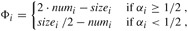
Figure 17.3: The effect of a sequence of n TABLE-INSERT operations on the number num_i of items in the table, the number size_i of slots in the table, and the potential Φ_i = 2·num_i - size_i, each being measured after the ith operation. The thin line shows num_i, the dashed line shows size_i, and the thick line shows Φ_i. Notice that immediately before an expansion, the potential has built up to the number of items in the table, and therefore it can pay for moving all the items to the new table. Afterwards, the potential drops to 0, but it is immediately increased by 2 when the item that caused the expansion is inserted.
Figure 17.4: The effect of a sequence of n TABLE-INSERT and TABLE-DELETE operations on the number num_i of items in the table, the number size_i of slots in the table, and the potential each being measured after the ith operation. The thin line shows num_i, the dashed line shows size_i, and the thick line shows Φ_i. Notice that immediately before an expansion, the potential has built up to the number of items in the table, and therefore it can pay for moving all the items to the new table. Likewise, immediately before a contraction, the potential has built up to the number of items in the table.

Chapter 18: B-Trees

Figure 18.1: A B-tree whose keys are the consonants of English. An internal node x containing n[x] keys has n[x] + 1 children. All leaves are at the same depth in the tree. The lightly shaded nodes are examined in a search for the letter R.
Figure 18.2: (a) A typical disk drive. It is composed of several platters that rotate around a spindle. Each platter is read and written with a head at the end of an arm. The arms are ganged together so that they move their heads in unison. Here, the arms rotate around a common pivot axis. A track is the surface that passes beneath the read/write head when it is stationary. (b) A cylinder consists of a set of covertical tracks.
Figure 18.3: A B-tree of height 2 containing over one billion keys. Each internal node and leaf contains 1000 keys. There are 1001 nodes at depth 1 and over one million leaves at depth 2. Shown inside each node x is n[x], the number of keys in x.
Figure 18.4: A B-tree of height 3 containing a minimum possible number of keys. Shown inside each node x is n[x].
Figure 18.5: Splitting a node with t = 4. Node y is split into two nodes, y and z, and the median key S of y is moved up into y's parent.
Figure 18.6: Splitting the root with t = 4. Root node r is split in two, and a new root node s is created. The new root contains the median key of r and has the two halves of r as children. The B-tree grows in height by one when the root is split.
Figure 18.7: Inserting keys into a B-tree. The minimum degree t for this B-tree is 3, so a node can hold at most 5 keys. Nodes that are modified by the insertion process are lightly shaded. (a) The initial tree for this example. (b) The result of inserting B into the initial tree; this is a simple insertion into a leaf node. (c) The result of inserting Q into the previous tree. The node RSTUV is split into two nodes containing RS and UV, the key T is moved up to the root, and Q is inserted in the leftmost of the two halves (the RS node). (d) The result of inserting L into the previous tree. The root is split right away, since it is full, and the B-tree grows in height by one. Then L is inserted into the leaf containing JK. (e) The result of inserting F into the previous tree. The node ABCDE is split before F is inserted into the rightmost of the two halves (the DE node).
Figure 18.8: Deleting keys from a B-tree. The minimum degree for this B-tree is t = 3, so a node (other than the root) cannot have fewer than 2 keys. Nodes that are modified are lightly shaded. (a) The B-tree of Figure 18.7(e). (b) Deletion of F. This is case 1: simple deletion from a leaf. (c) Deletion of M. This is case 2a: the predecessor L of M is moved up to take M's position. (d) Deletion of G. This is case 2c: G is pushed down to make node DEGJK, and then G is deleted from this leaf (case 1). (e) Deletion of D. This is case 3b: the recursion can't descend to node CL because it has only 2 keys, so P is pushed down and merged with CL and TX to form CLPTX; then, D is deleted from a leaf (case 1). (e′) After (d), the root is deleted and the tree shrinks in height by one. (f) Deletion of B. This is case 3a: C is moved to fill B's position and E is moved to fill C's position.

Chapter 19: Binomial Heaps

Figure 19.1: Running times for operations on three implementations of mergeable heaps. The number of items in the heap(s) at the time of an operation is denoted by n.
Figure 19.2: (a) The recursive definition of the binomial tree B_k. Triangles represent rooted subtrees. (b) The binomial trees B₀ through B₄. Node depths in B₄ are shown. (c) Another way of looking at the binomial tree B_k.
Figure 19.3: A binomial heap H with n = 13 nodes. (a) The heap consists of binomial trees B₀, B₂, and B₃, which have 1, 4, and 8 nodes respectively, totaling n = 13 nodes. Since each binomial tree is min-heap-ordered, the key of any node is no less than the key of its parent. Also shown is the root list, which is a linked list of roots in order of increasing degree. (b) A more detailed representation of binomial heap H . Each binomial tree is stored in the left-child, right-sibling representation, and each node stores its degree.
Figure 19.4: The binomial tree B₄ with nodes labeled in binary by a postorder walk.
Figure 19.5: The execution of BINOMIAL-HEAP-UNION. (a) Binomial heaps H₁ and H₂. (b) Binomial heap H is the output of BINOMIAL-HEAP-MERGE(H₁, H₂). Initially, x is the first root on the root list of H . Because both x and next-x have degree 0 and key[x] < key[next-x], case 3 applies. (c) After the link occurs, x is the first of three roots with the same degree, so case 2 applies. (d) After all the pointers move down one position in the root list, case 4 applies, since x is the first of two roots of equal degree. (e) After the link occurs, case 3 applies. (f) After another link, case 1 applies, because x has degree 3 and next-x has degree 4. This iteration of the while loop is the last, because after the pointers move down one position in the root list, next-x = NIL.
Figure 19.6: The four cases that occur in BINOMIAL-HEAP-UNION. Labels a, b, c, and d serve only to identify the roots involved; they do not indicate the degrees or keys of these roots. In each case, x is the root of a B_k-tree and l > k. (a) Case 1: degree[x] ≠ degree[next-x]. The pointers move one position farther down the root list. (b) Case 2: degree[x] = degree[next-x] = degree[sibling[next-x]]. Again, the pointers move one position farther down the list, and the next iteration executes either case 3 or case 4. (c) Case 3: degree[x] = degree[next-x] ≠ degree[sibling[next-x]] and key[x] ≤ key[next-x]. We remove next-x from the root list and link it to x, creating a B_k+1-tree. (d) Case 4: degree[x] = degree[next-x] ≠ degree[sibling[next-x]] and key[next-x] ≤ key[x]. We remove x from the root list and link it to next-x, again creating a B_k+1-tree.
Figure 19.7: The action of BINOMIAL-HEAP-EXTRACT-MIN. (a) A binomial heap H. (b) The root x with minimum key is removed from the root list of H . (c) The linked list of x's children is reversed, giving another binomial heap H′. (d) The result of uniting H and H'.
Figure 19.8: The action of BINOMIAL-HEAP-DECREASE-KEY. (a) The situation just before line 6 of the first iteration of the while loop. Node y has had its key decreased to 7, which is less than the key of y's parent z. (b) The keys of the two nodes are exchanged, and the situation just before line 6 of the second iteration is shown. Pointers y and z have moved up one level in the tree, but min-heap order is still violated. (c) After another exchange and moving pointers y and z up one more level, we find that min-heap order is satisfied, so the while loop terminates.

Chapter 20: Fibonacci Heaps

Figure 20.1: (a) A Fibonacci heap consisting of five min-heap-ordered trees and 14 nodes. The dashed line indicates the root list. The minimum node of the heap is the node containing the key 3. The three marked nodes are blackened. The potential of this particular Fibonacci heap is 5+2·3 = 11. (b) A more complete representation showing pointers p (up arrows), child (down arrows), and left and right (sideways arrows). These details are omitted in the remaining figures in this chapter, since all the information shown here can be determined from what appears in part (a).
Figure 20.2: Inserting a node into a Fibonacci heap. (a) A Fibonacci heap H. (b) Fibonacci heap H after the node with key 21 has been inserted. The node becomes its own min-heap-ordered tree and is then added to the root list, becoming the left sibling of the root.
Figure 20.3: The action of FIB-HEAP-EXTRACT-MIN. (a) A Fibonacci heap H. (b) The situation after the minimum node z is removed from the root list and its children are added to the root list. (c)–(e) The array A and the trees after each of the first three iterations of the for loop of lines 3–13 of the procedure CONSOLIDATE. The root list is processed by starting at the node pointed to by min[H ] and following right pointers. Each part shows the values of w and x at the end of an iteration. (f)–(h) The next iteration of the for loop, with the values of w and x shown at the end of each iteration of the while loop of lines 6–12. Part (f) shows the situation after the first time through the while loop. The node with key 23 has been linked to the node with key 7, which is now pointed to by x. In part (g), the node with key 17 has been linked to the node with key 7, which is still pointed to by x. In part (h), the node with key 24 has been linked to the node with key 7. Since no node was previously pointed to by A[3], at the end of the for loop iteration, A[3] is set to point to the root of the resulting tree. (i)–(l) The situation after each of the next four iterations of the for loop. (m) Fibonacci heap H after reconstruction of the root list from the array A and determination of the new min[H] pointer.
Figure 20.4: Two calls of FIB-HEAP-DECREASE-KEY. (a) The initial Fibonacci heap. (b) The node with key 46 has its key decreased to 15. The node becomes a root, and its parent (with key 24), which had previously been unmarked, becomes marked. (c)–(e) The node with key 35 has its key decreased to 5. In part (c), the node, now with key 5, becomes a root. Its parent, with key 26, is marked, so a cascading cut occurs. The node with key 26 is cut from its parent and made an unmarked root in (d). Another cascading cut occurs, since the node with key 24 is marked as well. This node is cut from its parent and made an unmarked root in part (e). The cascading cuts stop at this point, since the node with key 7 is a root. (Even if this node were not a root, the cascading cuts would stop, since it is unmarked.) The result of the FIB-HEAP-DECREASE-KEY operation is shown in part (e), with min[H] pointing to the new minimum node.

Chapter 21: Data Structures for Disjoint Sets

Figure 21.1: (a) A graph with four connected components: {a, b, c, d}, {e, f, g}, {h, i}, and {j}.(b) The collection of disjoint sets after each edge is processed.
Figure 21.2: (a) Linked-list representations of two sets. One contains objects b, c, e, and h, with c as the representative, and the other contains objects d, f, and g, with f as the representative. Each object on the list contains a set member, a pointer to the next object on the list, and a pointer back to the first object on the list, which is the representative. Each list has pointers head and tail to the first and last objects, respectively. (b) The result of UNION(e, g). The representative of the resulting set is f.
Figure 21.3: A sequence of 2n - 1 operations on n objects that takes Θ(n²) time, or Θ(n) time per operation on average, using the linked-list set representation and the simple implementation of UNION.
Figure 21.4: A disjoint-set forest. (a) Two trees representing the two sets of Figure 21.2. The tree on the left represents the set {b, c, e, h}, with c as the representative, and the tree on the right represents the set {d, f, g}, with f as the representative. (b) The result of UNION(e, g).
Figure 21.5: Path compression during the operation FIND-SET. Arrows and self-loops at roots are omitted. (a) A tree representing a set prior to executing FIND-SET(a). Triangles represent subtrees whose roots are the nodes shown. Each node has a pointer to its parent. (b) The same set after executing FIND-SET(a). Each node on the find path now points directly to the root.

Chapter 22: Elementary Graph Algorithms

Figure 22.1: Two representations of an undirected graph. (a) An undirected graph G having five vertices and seven edges. (b) An adjacency-list representation of G. (c) The adjacency-matrix representation of G.
Figure 22.2: Two representations of a directed graph. (a) A directed graph G having six vertices and eight edges. (b) An adjacency-list representation of G. (c) The adjacency-matrix representation of G.
Figure 22.3: The operation of BFS on an undirected graph. Tree edges are shown shaded as they are produced by BFS. Within each vertex u is shown d[u]. The queue Q is shown at the beginning of each iteration of the while loop of lines 10–18. Vertex distances are shown next to vertices in the queue.
Figure 22.4: The progress of the depth-first-search algorithm DFS on a directed graph. As edges are explored by the algorithm, they are shown as either shaded (if they are tree edges) or dashed (otherwise). Nontree edges are labeled B, C, or F according to whether they are back, cross, or forward edges. Vertices are timestamped by discovery time/finishing time.
Figure 22.5: Properties of depth-first search. (a) The result of a depth-first search of a directed graph. Vertices are timestamped and edge types are indicated as in Figure 22.4. (b) Intervals for the discovery time and finishing time of each vertex correspond to the parenthesization shown. Each rectangle spans the interval given by the discovery and finishing times of the corresponding vertex. Tree edges are shown. If two intervals overlap, then one is nested within the other, and the vertex corresponding to the smaller interval is a descendant of the vertex corresponding to the larger. (c) The graph of part (a) redrawn with all tree and forward edges going down within a depth-first tree and all back edges going up from a descendant to an ancestor.
Figure 22.6: A directed graph for use in Exercises 22.3-2 and 22.5-2.
Figure 22.7: (a) Professor Bumstead topologically sorts his clothing when getting dressed. Each directed edge (u, v) means that garment u must be put on before garment v. The discovery and finishing times from a depth-first search are shown next to each vertex. (b) The same graph shown topologically sorted. Its vertices are arranged from left to right in order of decreasing finishing time. Note that all directed edges go from left to right.
Figure 22.8: A dag for topological sorting.
Figure 22.9: (a) A directed graph G. The strongly connected components of G are shown as shaded regions. Each vertex is labeled with its discovery and finishing times. Tree edges are shaded. (b) The graph G^T, the transpose of G. The depth-first forest computed in line 3 of STRONGLY-CONNECTED-COMPONENTS is shown, with tree edges shaded. Each strongly connected component corresponds to one depth-first tree. Vertices b, c, g, and h, which are heavily shaded, are the roots of the depth-first trees produced by the depth-first search of G^T. (c) The acyclic component graph G^SCC obtained by contracting all edges within each strongly connected component of G so that only a single vertex remains in each component.
Figure 22.10: The articulation points, bridges, and biconnected components of a connected, undirected graph for use in Problem 22-2. The articulation points are the heavily shaded vertices, the bridges are the heavily shaded edges, and the biconnected components are the edges in the shaded regions, with a bcc numbering shown.

Chapter 23: Minimum Spanning Trees

Figure 23.1: A minimum spanning tree for a connected graph. The weights on edges are shown, and the edges in a minimum spanning tree are shaded. The total weight of the tree shown is 37. This minimum spanning tree is not unique: removing the edge (b, c) and replacing it with the edge (a, h) yields another spanning tree with weight 37.
Figure 23.2: Two ways of viewing a cut (S, V - S) of the graph from Figure 23.1. (a) The vertices in the set S are shown in black, and those in V - S are shown in white. The edges crossing the cut are those connecting white vertices with black vertices. The edge (d, c) is the unique light edge crossing the cut. A subset A of the edges is shaded; note that the cut (S, V - S) respects A, since no edge of A crosses the cut. (b) The same graph with the vertices in the set S on the left and the vertices in the set V - S on the right. An edge crosses the cut if it connects a vertex on the left with a vertex on the right.
Figure 23.3: The proof of Theorem 23.1. The vertices in S are black, and the vertices in V - S are white. The edges in the minimum spanning tree T are shown, but the edges in the graph G are not. The edges in A are shaded, and (u, v) is a light edge crossing the cut (S, V - S). The edge (x, y) is an edge on the unique path p from u to v in T. A minimum spanning tree T′ that contains (u, v) is formed by removing the edge (x, y) from T and adding the edge (u, v).
Figure 23.4: The execution of Kruskal's algorithm on the graph from Figure 23.1. Shaded edges belong to the forest A being grown. The edges are considered by the algorithm in sorted order by weight. An arrow points to the edge under consideration at each step of the algorithm. If the edge joins two distinct trees in the forest, it is added to the forest, thereby merging the two trees.
Figure 23.5: The execution of Prim's algorithm on the graph from Figure 23.1. The root vertex is a. Shaded edges are in the tree being grown, and the vertices in the tree are shown in black. At each step of the algorithm, the vertices in the tree determine a cut of the graph, and a light edge crossing the cut is added to the tree. In the second step, for example, the algorithm has a choice of adding either edge (b, c) or edge (a, h) to the tree since both are light edges crossing the cut.

Chapter 24: Single-Source Shortest Paths

Figure 24.1: Negative edge weights in a directed graph. Shown within each vertex is its shortest-path weight from source s. Because vertices e and f form a negative-weight cycle reachable from s, they have shortest-path weights of -∞. Because vertex g is reachable from a vertex whose shortest-path weight is -∞, it, too, has a shortest-path weight of -∞. Vertices such as h, i, and j are not reachable from s, and so their shortest-path weights are ∞, even though they lie on a negative-weight cycle.
Figure 24.2: (a) A weighted, directed graph with shortest-path weights from source s. (b) The shaded edges form a shortest-paths tree rooted at the source s. (c) Another shortest-paths tree with the same root.
Figure 24.3: Relaxation of an edge (u, v) with weight w(u, v) = 2. The shortest-path estimate of each vertex is shown within the vertex. (a) Because d[v] > d[u] + w(u, v) prior to relaxation, the value of d[v] decreases. (b) Here, d[v] ≤ d[u] + w(u, v) before the relaxation step, and so d[v] is unchanged by relaxation.
Figure 24.4: The execution of the Bellman-Ford algorithm. The source is vertex s. The d values are shown within the vertices, and shaded edges indicate predecessor values: if edge (u, v) is shaded, then π[v] = u. In this particular example, each pass relaxes the edges in the order (t, x), (t, y), (t, z), (x, t), (y, x), (y, z), (z, x), (z, s), (s, t), (s, y). (a) The situation just before the first pass over the edges. (b)–(e) The situation after each successive pass over the edges. The d and π values in part (e) are the final values. The Bellman-Ford algorithm returns TRUE in this example.
Figure 24.5: The execution of the algorithm for shortest paths in a directed acyclic graph. The vertices are topologically sorted from left to right. The source vertex is s. The d values are shown within the vertices, and shaded edges indicate the π values. (a) The situation before the first iteration of the for loop of lines 3–5. (b)–(g) The situation after each iteration of the for loop of lines 3–5. The newly blackened vertex in each iteration was used as u in that iteration. The values shown in part (g) are the final values.
Figure 24.6: The execution of Dijkstra's algorithm. The source s is the leftmost vertex. The shortest-path estimates are shown within the vertices, and shaded edges indicate predecessor values. Black vertices are in the set S, and white vertices are in the min-priority queue Q = V - S. (a) The situation just before the first iteration of the while loop of lines 4–8. The shaded vertex has the minimum d value and is chosen as vertex u in line 5. (b)-(f) The situation after each successive iteration of the while loop. The shaded vertex in each part is chosen as vertex u in line 5 of the next iteration. The d and π values shown in part (f) are the final values.
Figure 24.7: The proof of Theorem 24.6. Set S is nonempty just before vertex u is added to it. A shortest path p from source s to vertex u can be decomposed into s , where y is the first vertex on the path that is not in S and x ∈ S immediately precedes y. Vertices x and y are distinct, but we may have s = x or y = u. Path p₂ may or may not reenter set S.
Figure 24.8: The constraint graph corresponding to the system (24.3)–(24.10) of difference constraints. The value of δ(v₀, v_i) is shown in each vertex v_i. A feasible solution to the system is x = (-5, -3, 0, -1, -4).
Figure 24.9: Showing that a path in G_π from source s to vertex v is unique. If there are two paths and , where x ≠ y, then π[z] = x and π[z] = y, a contradiction.

Chapter 25: All-Pairs Shortest Paths

Figure 25.1: A directed graph and the sequence of matrices L^(m) computed by SLOW-ALL-PAIRS-SHORTEST-PATHS. The reader may verify that L⁽⁵⁾ = L⁽⁴⁾ · W is equal to L⁽⁴⁾, and thus L^(m) = L⁽⁴⁾ for all m ≥ 4.
Figure 25.2: A weighted, directed graph for use in Exercises 25.1-1, 25.2-1, and 25.3-1.
Figure 25.3: Path p is a shortest path from vertex i to vertex j, and k is the highest-numbered intermediate vertex of p. Path p₁, the portion of path p from vertex i to vertex k, has all intermediate vertices in the set {1, 2,..., k - 1}. The same holds for path p₂ from vertex k to vertex j.
Figure 25.4: The sequence of matrices D^(k) and Π^(k) computed by the Floyd-Warshall algorithm for the graph in Figure 25.1.
Figure 25.5: A directed graph and the matrices T^(k) computed by the transitive-closure algorithm.
Figure 25.6: Johnson's all-pairs shortest-paths algorithm run of the graph of Figure 25.1. (a) The graph G′ with the original weight function w. The new vertex s is black. Within each vertex v is h(v) = δ(s, v). (b) Each edge (u, v) is reweighted with weight function . (c)–(g) The result of running Dijkstra's algorithm on each vertex of G using weight function . In each part, the source vertex u is black, and shaded edges are in the shortest-paths tree computed by the algorithm. Within each vertex v are the values and δ(u, v), separated by a slash. The value d_uv = δ(u, v) is equal to .

Chapter 26: Maximum Flow

Figure 26.1: (a) A flow network G = (V, E) for the Lucky Puck Company's trucking problem. The Vancouver factory is the source s, and the Winnipeg warehouse is the sink t. Pucks are shipped through intermediate cities, but only c(u, v) crates per day can go from city u to city v. Each edge is labeled with its capacity. (b) A flow f in G with value |f| = 19. Only positive flows are shown. If f (u, v) > 0, edge (u, v) is labeled by f(u, v)/c(u, v). (The slash notation is used merely to separate the flow and capacity; it does not indicate division.) If f(u, v) ≤ 0, edge (u, v) is labeled only by its capacity.
Figure 26.2: Converting a multiple-source, multiple-sink maximum-flow problem into a problem with a single source and a single sink. (a) A flow network with five sources S = {s₁, s₂, s₃, s₄, s₅} and three sinks T = {t₁, t₂, t₃}. (b) An equivalent single-source, single-sink flow network. We add a supersource s and an edge with infinite capacity from s to each of the multiple sources. We also add a supersink t and an edge with infinite capacity from each of the multiple sinks to t.
Figure 26.3: (a) The flow network G and flow f of Figure 26.1(b). (b) The residual network G_f with augmenting path p shaded; its residual capacity is c_f (p) = c(v₂, v₃) = 4. (c) The flow in G that results from augmenting along path p by its residual capacity 4. (d) The residual network induced by the flow in (c).
Figure 26.4: A cut (S, T) in the flow network of Figure 26.1(b), where S = {s, v₁, v₂} and T = {v₃, v₄, t}. The vertices in S are black, and the vertices in T are white. The net flow across (S, T) is f(S, T) = 19, and the capacity is c(S, T) = 26.
Figure 26.5: The execution of the basic Ford-Fulkerson algorithm. (a)–(d) Successive iterations of the while loop. The left side of each part shows the residual network G_f from line 4 with a shaded augmenting path p. The right side of each part shows the new flow f that results from adding f_p to f. The residual network in (a) is the input network G. (e) The residual network at the last while loop test. It has no augmenting paths, and the flow f shown in (d) is therefore a maximum flow.
Figure 26.6: (a) A flow network for which FORD-FULKERSON can take Θ(E |f*|) time, where f* is a maximum flow, shown here with |f*| = 2,000,000. An augmenting path with residual capacity 1 is shown. (b) The resulting residual network. Another augmenting path with residual capacity 1 is shown. (c) The resulting residual network.
Figure 26.7: A bibartite graph G = (V, E) with vertex partition V = L∪R. (a) A matching with cardinality 2. (b) A maximum matching with cardinality 3.
Figure 26.8: The flow network corresponding to a bipartite graph. (a) The bipartite graph G = (V, E) with vertex partition V = L ∪ R from Figure 26.7. A maximum matching is shown by shaded edges. (b) The corresponding flow network G' with a maximum flow shown. Each edge has unit capacity. Shaded edges have a flow of 1, and all other edges carry no flow. The shaded edges from L to R correspond to those in a maximum matching of the bipartite graph.
Figure 26.9: Discharging a vertex y. It takes 15 iterations of the while loop of DISCHARGE to push all the excess flow from y. Only the neighbors of y and edges entering or leaving y are shown. In each part, the number inside each vertex is its excess at the beginning of the first iteration shown in the part, and each vertex is shown at its height throughout the part. To the right is shown the neighbor list N[y] at the beginning of each iteration, with the iteration number on top. The shaded neighbor is current[y]. (a) Initially, there are 19 units of excess to push from y, and current[y] = s. Iterations 1, 2, and 3 just advance current[y], since there are no admissible edges leaving y. In iteration 4, current[y] = NIL (shown by the shading being below the neighbor list), and so y is relabeled and current[y] is reset to the head of the neighbor list. (b) After relabeling, vertex y has height 1. In iterations 5 and 6, edges (y, s) and (y, x) are found to be inadmissible, but 8 units of excess flow are pushed from y to z in iteration 7. Because of the push, current[y] is not advanced in this iteration. (c) Because the push in iteration 7 saturated edge (y, z), it is found inadmissible in iteration 8. In iteration 9, current[y] = NIL, and so vertex y is again relabeled and current[y] is reset. (d) In iteration 10, (y, s) is inadmissible, but 5 units of excess flow are pushed from y to x in iteration 11. (e) Because current[y] was not advanced in iteration 11, iteration 12 finds (y, x) to be inadmissible. Iteration 13 finds (y, z) inadmissible, and iteration 14 relabels vertex y and resets current[y]. (f) Iteration 15 pushes 6 units of excess flow from y to s. (g) Vertex y now has no excess flow, and DISCHARGE terminates. In this example, DISCHARGE both starts and finishes with the current pointer at the head of the neighbor list, but in general this need not be the case.
Figure 26.10: The action of RELABEL-TO-FRONT. (a) A flow network just before the first iteration of the while loop. Initially, 26 units of flow leave source s. On the right is shown the initial list L = 〉x, y, z〉, where initially u = x. Under each vertex in list L is its neighbor list, with the current neighbor shaded. Vertex x is discharged. It is relabeled to height 1, 5 units of excess flow are pushed to y, and the 7 remaining units of excess are pushed to the sink t. Because x is relabeled, it is moved to the head of L, which in this case does not change the structure of L. (b) After x, the next vertex in L that is discharged is y. Figure 26.9 shows the detailed action of discharging y in this situation. Because y is relabeled, it is moved to the head of L. (c) Vertex x now follows y in L, and so it is again discharged, pushing all 5 units of excess flow to t. Because vertex x is not relabeled in this discharge operation, it remains in place in list L. (d) Since vertex z follows vertex x in L, it is discharged. It is relabeled to height 1 and all 8 units of excess flow are pushed to t. Because z is relabeled, it is moved to the front of L. (e) Vertex y now follows vertex z in L and is therefore discharged. But because y has no excess, DISCHARGE immediately returns, and y remains in place in L. Vertex x is then discharged. Because it, too, has no excess, DISCHARGE again returns, and x remains in place in L. RELABEL-TO-FRONT has reached the end of list L and terminates. There are no overflowing vertices, and the preflow is a maximum flow.
Figure 26.11: Grids for the escape problem. Starting points are black, and other grid vertices are white. (a) A grid with an escape, shown by shaded paths. (b) A grid with no escape.

Chapter 27: Sorting Networks

Figure 27.1: (a) A comparator with inputs x and y and outputs x' and y'. (b) The same comparator, drawn as a single vertical line. Inputs x = 7, y = 3 and outputs x' = 3, y' = 7 are shown.
Figure 27.2: (a) A 4-input, 4-output comparison network, which is in fact a sorting network. At time 0, the input values shown appear on the four input wires. (b) At time 1, the values shown appear on the outputs of comparators A and B, which are at depth 1. (c) At time 2, the values shown appear on the outputs of comparators C and D, at depth 2. Output wires b₁ and b₄ now have their final values, but output wires b₂ and b₃ do not. (d) At time 3, the values shown appear on the outputs of comparator E, at depth 3. Output wires b₂ and b₃ now have their final values.
Figure 27.3: A sorting network based on insertion sort for use in Exercise 27.1-6.
Figure 27.4: The operation of the comparator in the proof of Lemma 27.1. The function f is monotonically increasing.
Figure 27.5: (a) The sorting network from Figure 27.2 with input sequence 〈9, 5, 2, 6〉. (b) The same sorting network with the monotonically increasing function f(x) = f(⌈x/2⌉) applied to the inputs. Each wire in this network has the value of f applied to the value on the corresponding wire in (a).
Figure 27.6: A sorting network for sorting 4 numbers.
Figure 27.7: The comparison network HALF-CLEANER[8]. Two different sample zero-one input and output values are shown. The input is assumed to be bitonic. A half-cleaner ensures that every output element of the top half is at least as small as every output element of the bottom half. Moreover, both halves are bitonic, and at least one half is clean.
Figure 27.8: The possible comparisons in HALF-CLEANER[n]. The input sequence is assumed to be a bitonic sequence of 0's and 1's, and without loss of generality, we assume that it is of the form 00 ... 011 ... 100 ... 0. Subsequences of 0's are white, and subsequences of 1's are gray. We can think of the n inputs as being divided into two halves such that for i = 1, 2,..., n/2, inputs i and i + n/2 are compared. (a)–(b) Cases in which the division occurs in the middle subsequence of 1's. (c)–(d) Cases in which the division occurs in a subsequence of 0's. For all cases, every element in the top half of the output is at least as small as every element in the bottom half, both halves are bitonic, and at least one half is clean.
Figure 27.9: The comparison network BITONIC-SORTER[n], shown here for n = 8. (a) The recursive construction: HALF-CLEANER[n] followed by two copies of BITONIC-SORTER[n/2] that operate in parallel. (b) The network after unrolling the recursion. Each half-cleaner is shaded. Sample zero-one values are shown on the wires.
Figure 27.10: Comparing the first stage of MERGER[n] with HALF-CLEANER[n], for n = 8. (a) The first stage of MERGER[n] transforms the two monotonic input sequences 〈a₁, a₂,...,a_n/2〉 and 〈a_n/2+1, a_n/2+2,...,a_n〉 into two bitonic sequences 〈b₁, b₂,...,b_n/2〉 and 〈b_n/2+1, b_n/2+2,...,b_n〉. (b) The equivalent operation for HALF-CLEANER[n]. The bitonic input sequence 〈a₁, a₂,...,a_n/2-1, a_n/2, a_n, a_n-1,...,a_n/2+2, a_n/2+1〉 is transformed into the two bitonic sequences 〈b₁, b₂,...,b_n/2〉 and 〈b_n, b_n-1,...,b_n/2+1〉.
Figure 27.11: A network that merges two sorted input sequences into one sorted output sequence. The network MERGER[n] can be viewed as BITONIC-SORTER[n] with the first half-cleaner altered to compare inputs i and n - i + 1 for i = 1, 2,..., n/2. Here, n = 8. (a) The network decomposed into the first stage followed by two parallel copies of BITONIC-SORTER[n/2]. (b) The same network with the recursion unrolled. Sample zero-one values are shown on the wires, and the stages are shaded.
Figure 27.12: The sorting network SORTER[n] constructed by recursively combining merging networks. (a) The recursive construction. (b) Unrolling the recursion. (c) Replacing the MERGER boxes with the actual merging networks. The depth of each comparator is indicated, and sample zero-one values are shown on the wires.
Figure 27.13: An odd-even sorting network on 8 inputs.
Figure 27.14: Permutation networks. (a) The permutation network P₂, which consists of a single switch that can be set in either of the two ways shown. (b) The recursive construction of P₈ from 8 switches and two P₄'s. The switches and P₄'s are set to realize the permutation π = 〈4, 7,3, 5,1, 6, 8, 2〉.

Chapter 28: Matrix Operations

Figure 28.1: The operation of LU-DECOMPOSITION. (a) The matrix A. (b) The element a₁₁ = 2 in the black circle is the pivot, the shaded column is v/a₁₁, and the shaded row is w^T. The elements of U computed thus far are above the horizontal line, and the elements of L are to the left of the vertical line. The Schur complement matrix A′ - vw^T/a₁₁ occupies the lower right. (c) We now operate on the Schur complement matrix produced from part (b). The element a₂₂ = 4 in the black circle is the pivot, and the shaded column and row are v/a₂₂ and w^T (in the partitioning of the Schur complement), respectively. Lines divide the matrix into the elements of U computed so far (above), the elements of L computed so far (left), and the new Schur complement (lower right). (d) The next step completes the factorization. (The element 3 in the new Schur complement becomes part of U when the recursion terminates.) (e) The factorization A = LU.
Figure 28.2: The operation of LUP-DECOMPOSITION. (a) The input matrix A with the identity permutation of the rows on the left. The first step of the algorithm determines that the element 5 in the black circle in the third row is the pivot for the first column. (b) Rows 1 and 3 are swapped and the permutation is updated. The shaded column and row represent v and w^T. (c) The vector v is replaced by v/5, and the lower right of the matrix is updated with the Schur complement. Lines divide the matrix into three regions: elements of U (above), elements of L (left), and elements of the Schur complement (lower right). (d)–(f) The second step. (g)–(i) The third step. No further changes occur on the fourth, and final, step. (j) The LUP decomposition PA = LU.
Figure 28.3: The least-squares fit of a quadratic polynomial to the set of five data points {(-1, 2), (1, 1), (2, 1), (3, 0), (5,3)}. The black dots are the data points, and the white dots are their estimated values predicted by the polynomial F(x) = 1.2 - 0.757x + 0.214x², the quadratic polynomial that minimizes the sum of the squared errors. The error for each data point is shown as a shaded line.

Chapter 29: Linear Programming

Figure 29.1: The effects of policies on voters. Each entry describes the number of thousands of urban, suburban, or rural voters who could be won over by spending $1,000 on advertising support of a policy on a particular issue. Negative entries denote votes that would be lost.
Figure 29.2: (a) The linear program given in (29.12)–(29.15). Each constraint is represented by a line and a direction. The intersection of the constraints, which is the feasible region, is shaded. (b) The dotted lines show, respectively, the points for which the objective value is 0, 4, and 8. The optimal solution to the linear program is x₁ = 2 and x₂ = 6 with objective value 8.
Figure 29.3: (a) An example of a minimum-cost-flow problem. We denote the capacities by c and the costs by a. Vertex s is the source and vertex t is the sink, and we wish to send 4 units of flow from s to t. (b) A solution to the minimum-cost flow problem in which 4 units of flow are sent from s to t. For each edge, the flow and capacity are written as flow/capacity.

Chapter 30: Polynomials and the FFT

Figure 30.1: A graphical outline of an efficient polynomial-multiplication process. Representations on the top are in coefficient form, while those on the bottom are in point-value form. The arrows from left to right correspond to the multiplication operation. The w_2n terms are complex (2n)th roots of unity.
Figure 30.2: The values of in the complex plane, where w₈ = e^πi/8 is the principal 8th root of unity.
Figure 30.3: A butterfly operation. (a) The two input values enter from the left, the twiddle factor is multiplied by , and the sum and difference are output on the right. (b) A simplified drawing of a butterfly operation. We will use this representation in a parallel FFT circuit.
Figure 30.4: The tree of input vectors to the recursive calls of the RECURSIVE-FFT procedure. The initial invocation is for n = 8.
Figure 30.5: A circuit PARALLEL-FFT that computes the FFT, here shown on n = 8 inputs. Each butterfly operation takes as input the values on two wires, along with a twiddle factor, and it produces as outputs the values on two wires. The stages of butterflies are labeled to correspond to iterations of the outermost loop of the ITERATIVE-FFT procedure. Only the top and bottom wires passing through a butterfly interact with it; wires that pass through the middle of a butterfly do not affect that butterfly, nor are their values changed by that butterfly. For example, the top butterfly in stage 2 has nothing to do with wire 1 (the wire whose output is labeled y₁); its inputs and outputs are only on wires 0 and 2 (labeled y₀ and y₂, respectively). An FFT on n inputs can be computed in Θ(lg n) depth with Θ(n lg n) butterfly operations.

Chapter 31: Number-Theoretic Algorithms

Figure 31.1: An example of the operation of EXTENDED-EUCLID on the inputs 99 and 78. Each line shows one level of the recursion: the values of the inputs a and b, the computed value ⌊a/b⌋, and the values d, x, and y returned. The triple (d, x, y) returned becomes the triple (d′, x′, y′) used in the computation at the next higher level of recursion. The call EXTENDED-EUCLID(99, 78) returns (3, -11, 14), so gcd(99, 78) = 3 and gcd(99, 78) = 3 = 99 · (-11) + 78 · 14.
Figure 31.2: Two finite groups. Equivalence classes are denoted by their representative elements. (a) The group (Z₆, +₆). (b) The group ().
Figure 31.3: An illustration of the Chinese remainder theorem for n₁ = 5 and n₂ = 13. For this example, c₁ = 26 and c₂ = 40. In row i, column j is shown the value of a, modulo 65, such that (a mod 5) = i and (a mod 13) = j. Note that row 0, column 0 contains a 0. Similarly, row 4,column 12 contains a 64 (equivalent to -1). Since c₁ = 26, moving down a row increases a by 26. Similarly, c₂ = 40 means that moving right by a column increases a by 40. Increasing a by 1 corresponds to moving diagonally downward and to the right, wrapping around from the bottom to the top and from the right to the left.
Figure 31.4: The results of MODULAR-EXPONENTIATION when computing a^b (mod n), where a = 7, b = 560 = 〈1000110000〉, and n = 561. The values are shown after each execution of the for loop. The final result is 1.
Figure 31.5: Encryption in a public key system. Bob encrypts the message M using Alice's public key P_A and transmits the resulting ciphertext C = P_A(M) to Alice. An eavesdropper who captures the transmitted ciphertext gains no information about M. Alice receives C and decrypts it using her secret key to obtain the original message M = S_A(C).
Figure 31.6: Digital signatures in a public-key system. Alice signs the message M′ by appending her digital signature Σ = S_A(M′) to it. She transmits the message/signature pair (M′, Σ) to Bob, who verifies it by checking the equation M′ = P_A(Σ). If the equation holds, he accepts (M′, Σ) as a message that has been signed by Alice.
Figure 31.7: Pollard's rho heuristic. (a) The values produced by the recurrence mod 1387, starting with x₁ = 2. The prime factorization of 1387 is 19 · 73. The heavy arrows indicate the iteration steps that are executed before the factor 19 is discovered. The light arrows point to unreached values in the iteration, to illustrate the "rho" shape. The shaded values are the y values stored by POLLARD-RHO. The factor 19 is discovered upon reaching x₇ = 177, when gcd(63 - 177, 1387) = 19 is computed. The first x value that would be repeated is 1186, but the factor 19 is discovered before this value is repeated. (b) The values produced by the same recurrence, modulo 19. Every value x_i given in part (a) is equivalent, modulo 19, to the value shown here. For example, both x₄ = 63 and x₇ = 177 are equivalent to 6, modulo 19. (c) The values produced by the same recurrence, modulo 73. Every value x_i given in part (a) is equivalent, modulo 73, to the value shown here. By the Chinese remainder theorem, each node in part (a) corresponds to a pair of nodes, one from part (b) and one from part (c).

Chapter 32: String Matching

Figure 32.1: The string-matching problem. The goal is to find all occurrences of the pattern P = abaa in the text T = abcabaabcabac. The pattern occurs only once in the text, at shift s = 3. The shift s = 3 is said to be a valid shift. Each character of the pattern is connected by a vertical line to the matching character in the text, and all matched characters are shown shaded.
Figure 32.2: The string-matching algorithms in this chapter and their preprocessing and matching times.
Figure 32.3: A graphical proof of Lemma 32.1. We suppose that x ⊐ z and y ⊐ z. The three parts of the figure illustrate the three cases of the lemma. Vertical lines connect matching regions (shown shaded) of the strings. (a) If |x| ≤ |y|, then x ⊐ y. (b) If |x| ≥ |y|, then y ⊐ x. (c) If |x| = |y|, then x = y.
Figure 32.4: The operation of the naive string matcher for the pattern P = aab and the text T = acaabc. We can imagine the pattern P as a "template" that we slide next to the text. (a)–(d) The four successive alignments tried by the naive string matcher. In each part, vertical lines connect corresponding regions found to match (shown shaded), and a jagged line connects the first mismatched character found, if any. One occurrence of the pattern is found, at shift s = 2, shown in part (c).
Figure 32.5: The Rabin-Karp algorithm. Each character is a decimal digit, and we compute values modulo 13. (a) A text string. A window of length 5 is shown shaded. The numerical value of the shaded number is computed modulo 13, yielding the value 7. (b) The same text string with values computed modulo 13 for each possible position of a length-5 window. Assuming the pattern P = 31415, we look for windows whose value modulo 13 is 7, since 31415 ≡ 7 (mod 13). Two such windows are found, shown shaded in the figure. The first, beginning at text position 7, is indeed an occurrence of the pattern, while the second, beginning at text position 13, is a spurious hit. (c) Computing the value for a window in constant time, given the value for the previous window. The first window has value 31415. Dropping the high-order digit 3, shifting left (multiplying by 10), and then adding in the low-order digit 2 gives us the new value 14152. All computations are performed modulo 13, however, so the value for the first window is 7, and the value computed for the new window is 8.
Figure 32.6: A simple two-state finite automaton with state set Q = {0, 1}, start state q₀ = 0, and input alphabet Σ = {a, b}. (a) A tabular representation of the transition function δ. (b) An equivalent state-transition diagram. State 1 is the only accepting state (shown blackened). Directed edges represent transitions. For example, the edge from state 1 to state 0 labeled b indicates δ(1, b) = 0. This automaton accepts those strings that end in an odd number of a's. More precisely, a string x is accepted if and only if x = yz, where y = ε or y ends with a b, and z = a^k, where k is odd. For example, the sequence of states this automaton enters for input abaaa (including the start state) is 〈0, 1, 0, 1, 0, 1〉, and so it accepts this input. For input abbaa, the sequence of states is 〈0, 1, 0, 0, 1, 0〉, and so it rejects this input.
Figure 32.7: (a) A state-transition diagram for the string-matching automaton that accepts all strings ending in the string ababaca. State 0 is the start state, and state 7 (shown blackened) is the only accepting state. A directed edge from state i to state j labeled a represents δ(i, a) = j. The right-going edges forming the "spine" of the automaton, shown heavy in the figure, correspond to successful matches between pattern and input characters. The left-going edges correspond to failing matches. Some edges corresponding to failing matches are not shown; by convention, if a state i has no outgoing edge labeled a for some a ∈ Σ, then δ(i, a) = 0. (b) The corresponding transition function δ, and the pattern string P = ababaca. The entries corresponding to successful matches between pattern and input characters are shown shaded. (c) The operation of the automaton on the text T = abababacaba. Under each text character T [i] is given the state φ(T_i) the automaton is in after processing the prefix T_i. One occurrence of the pattern is found, ending in position 9.
Figure 32.8: An illustration for the proof of Lemma 32.2. The figure shows that r ≤ σ(x) + 1, where r = σ(xa).
Figure 32.9: An illustration for the proof of Lemma 32.3. The figure shows that r = σ(P_qa), where q = σ(x) and r = σ(xa).
Figure 32.10: The prefix function π. (a) The pattern P = ababaca is aligned with a text T so that the first q = 5 characters match. Matching characters, shown shaded, are connected by vertical lines. (b) Using only our knowledge of the 5 matched characters, we can deduce that a shift of s + 1 is invalid, but that a shift of s′ = s + 2 is consistent with everything we know about the text and therefore is potentially valid. (c) The useful information for such deductions can be precomputed by comparing the pattern with itself. Here, we see that the longest prefix of P that is also a proper suffix of P₅ is P₃. This information is precomputed and represented in the array π, so that π[5] = 3. Given that q characters have matched successfully at shift s, the next potentially valid shift is at s′ = s + (q - π[q]).
Figure 32.11: An illustration of Lemma 32.5 for the pattern P = ababababca and q = 8. (a) The π function for the given pattern. Since π[8] = 6, π[6] = 4, π[4] = 2, and π[2] = 0, by iterating π we obtain π*[8] = {6, 4, 2, 0}. (b) We slide the template containing the pattern P to the right and note when some prefix P_k of P matches up with some proper suffix of P₈; this happens for k = 6, 4, 2, and 0. In the figure, the first row gives P, and the dotted vertical line is drawn just after P₈. Successive rows show all the shifts of P that cause some prefix P_k of P to match some suffix of P₈. Successfully matched characters are shown shaded. Vertical lines connect aligned matching characters. Thus, {k : k < q and P_k ⊐ P_q} = {6, 4,2, 0}. The lemma claims that π*[q] = {k : k < q and P_k ⊐ P_q} for all q.

Chapter 33: Computational Geometry

Figure 33.1: (a) The cross product of vectors p₁ and p₂ is the signed area of the parallelogram. (b) The lightly shaded region contains vectors that are clockwise from p. The darkly shaded region contains vectors that are counterclockwise from p.
Figure 33.2: Using the cross product to determine how consecutive line segments and turn at point p₁. We check whether the directed segment is clockwise or counterclockwise relative to the directed segment . (a) If counterclockwise, the points make a left turn. (b) If clockwise, they make a right turn.
Figure 33.3: Cases in the procedure SEGMENTS-INTERSECT. (a) The segments and straddle each other's lines. Because straddles the line containing , the signs of the cross products (p₃ - p₁) × (p₂ - p₁) and (p₄ - p₁) × (p₂ - p₁) differ. Because straddles the line containing , the signs of the cross products (p₁ - p₃) × (p₄ - p₃) and (p₂ - p₃) × (p₄ - p₃) differ. (b) Segment straddles the line containing , but does not straddle the line containing . The signs of the cross products (p₁ - p₃) × (p₄ - p₃) and (p₂ - p₃) × (p₄ - p₃) are the same. (c) Point p₃ is collinear with and is between p₁ and p₂. (d) Point p₃ is collinear with , but it is not between p₁ and p₂. The segments do not intersect.
Figure 33.4: The ordering among line segments at various vertical sweep lines. (a) We have a >_r c, a >_t b, b >_t c, a >_r c, and b >_u c. Segment d is comparable with no other segment shown. (b) When segments e and f intersect, their orders are reversed: we have e >_v f but f >_w e. Any sweep line (such as z) that passes through the shaded region has e and f consecutive in its total order.
Figure 33.5: The execution of ANY-SEGMENTS-INTERSECT. Each dashed line is the sweep line at an event point, and the ordering of segment names below each sweep line is the total order T at the end of the for loop in which the corresponding event point is processed. The intersection of segments d and b is found when segment c is deleted.
Figure 33.6: A set of points Q = {p₀, p₁, ..., p₁₂} with its convex hull CH(Q) in gray.
Figure 33.7: The execution of GRAHAM-SCAN on the set Q of Figure 33.6. The current convex hull contained in stack S is shown in gray at each step. (a) The sequence 〈 p₁, p₂, ..., p₁₂〉 of points numbered in order of increasing polar angle relative to p₀, and the initial stack S containing p₀, p₁, and p₂. (b)–(k) Stack S after each iteration of the for loop of lines 6–9. Dashed lines show nonleft turns, which cause points to be popped from the stack. In part (h), for example, the right turn at angle ∠p₇p₈p₉ causes p₈ to be popped, and then the right turn at angle ∠p₆p₇p₉ causes p₇ to be popped. (l) The convex hull returned by the procedure, which matches that of Figure 33.6.
Figure 33.8: The proof of correctness of GRAHAM-SCAN. (a) Because p_i's polar angle relative to p₀ is greater than p_j's polar angle, and because the angle ∠p_kp_j p_i makes a left turn, adding p_i to CH(Q_j) gives exactly the vertices of CH(Q_j ∪{p_i}). (b) If the angle ∠p_rp_tp_i makes a nonleft turn, then p_t is either in the interior of the triangle formed by p₀, p_r, and p_i or on a side of the triangle, and it cannot be a vertex of CH(Q_i).
Figure 33.9: The operation of Jarvis's march. The first vertex chosen is the lowest point p₀. The next vertex, p₁, has the smallest polar angle of any point with respect to p₀. Then, p₂ has the smallest polar angle with respect to p₁. The right chain goes as high as the highest point p₃. Then, the left chain is constructed by finding smallest polar angles with respect to the negative x-axis.
Figure 33.10: The definition of a star-shaped polygon, for use in Exercise 33.3-4. (a) A star-shaped polygon. The segment from point p to any point q on the boundary intersects the boundary only at q. (b) A non-star-shaped polygon. The shaded region on the left is the shadow of q, and the shaded region on the right is the shadow of q′. Since these regions are disjoint, the kernel is empty.
Figure 33.11: Key concepts in the proof that the closest-pair algorithm needs to check only 7 points following each point in the array Y′. (a) If p_L ∈ P_L and p_R ∈ P_R are less than δ units apart, they must reside within a δ × 2δ rectangle centered at line l. (b) How 4 points that are pairwise at least δ units apart can all reside within a δ × δ square. On the left are 4 points in P_L, and on the right are 4 points in P_R. There can be 8 points in the δ × 2δ rectangle if the points shown on line l are actually pairs of coincident points with one point in P_L and one in P_R.

Chapter 34: NP-Completeness

Figure 34.1: Using a polynomial-time reduction algorithm to solve a decision problem A in polynomial time, given a polynomial-time decision algorithm for another problem B. In polynomial time, we transform an instance α of A into an instance β of B, we solve B in polynomial time, and we use the answer for β as the answer for α.
Figure 34.2: (a) A graph representing the vertices, edges, and faces of a dodecahedron, with a hamiltonian cycle shown by shaded edges. (b) A bipartite graph with an odd number of vertices. Any such graph is nonhamiltonian.
Figure 34.3: Four possibilities for relationships among complexity classes. In each diagram, one region enclosing another indicates a proper-subset relation. (a) P = NP = co-NP. Most researchers regard this possibility as the most unlikely. (b) If NP is closed under complement, then NP = co-NP, but it need not be the case that P = NP. (c) P = NP ∪ co-NP, but NP is not closed under complement. (d) NP ≠ co-NP and P ≠ NP ∪ co-NP. Most researchers regard this possibility as the most likely.
Figure 34.4: An illustration of a polynomial-time reduction from a language L₁ to a language L₂ via a reduction function f. For any input x ∈ {0, 1}*, the question of whether x ∈ L₁ has the same answer as the question of whether f(x) ∈ L₂.
Figure 34.5: The proof of Lemma 34.3. The algorithm F is a reduction algorithm that computes the reduction function f from L₁ to L₂ in polynomial time, and A₂ is a polynomial-time algorithm that decides L₂. Illustrated is an algorithm A1 that decides whether x ∈ L₁ by using F to transform any input x into f (x) and then using A₂ to decide whether f(x) ∈ L₂.
Figure 34.6: How most theoretical computer scientists view the relationships among P, NP, and NPC. Both P and NPC are wholly contained within NP, and P ∩ NPC = Ø.
Figure 34.7: Three basic logic gates, with binary inputs and outputs. Under each gate is the truth table that describes the gate's operation. (a) The NOT gate. (b) The AND gate. (c) The OR gate.
Figure 34.8: Two instances of the circuit-satisfiability problem. (a) The assignment 〈x₁ = 1, x₂ = 1, x₃ = 0〉 to the inputs of this circuit causes the output of the circuit to be 1. The circuit is therefore satisfiable. (b) No assignment to the inputs of this circuit can cause the output of the circuit to be 1. The circuit is therefore unsatisfiable.
Figure 34.9: The sequence of configurations produced by an algorithm A running on an input x and certificate y. Each configuration represents the state of the computer for one step of the computation and, besides A, x, and y, includes the program counter (PC), auxiliary machine state, and working storage. Except for the certificate y, the initial configuration c₀ is constant. Each configuration is mapped to the next configuration by a boolean combinational circuit M. The output is a distinguished bit in the working storage.
Figure 34.10: Reducing circuit satisfiability to formula satisfiability. The formula produced by the reduction algorithm has a variable for each wire in the circuit.
Figure 34.11: The tree corresponding to the formula φ = ((x₁ → x₂)⊦¬((¬x₁ ↔ x₃)⊦ x₄))⊥¬x₂.
Figure 34.12: The truth table for the clause (y₁ ↔ (y₂ ⊥ ¬x₂)).
Figure 34.13: The structure of NP-completeness proofs in Sections 34.4 and 34.5. All proofs ultimately follow by reduction from the NP-completeness of CIRCUIT-SAT.
Figure 34.14: The graph G derived from the 3-CNF formula φ = C₁ ⊥ C₂ ⊥ C₃, where C₁ = (x₁ ⊦ ¬x₂ ⊦ ¬x₃), C₂ = (¬x₁ ⊥ x₂ ⊥ x₃), and C₃ = (x₁ ⊥ x₂ ⊥ x₃), in reducing 3-CNF-SAT to CLIQUE. A satisfying assignment of the formula has x₂ = 0, x₃ = 1, and x₁ may be either 0 or 1. This assignment satisfies C₁ with ¬x₂, and it satisfies C₂ and C₃ with x₃, corresponding to the clique with lightly shaded vertices.
Figure 34.15: Reducing CLIQUE to VERTEX-COVER. (a) An undirected graph G = (V, E) with clique V' = {u, v, x, y}. (b) The graph produced by the reduction algorithm that has vertex cover V - V' = {w, z}.
Figure 34.16: The widget used in reducing the vertex-cover problem to the hamiltonian-cycle problem. An edge (u, v) of graph G corresponds to widget W_uv in the graph G' created in the reduction. (a) The widget, with individual vertices labeled. (b)–(d) The shaded paths are the only possible ones through the widget that include all vertices, assuming that the only connections from the widget to the remainder of G' are through vertices [u, v, 1], [u, v, 6], [v, u, 1], and [v, u, 6].
Figure 34.17: The reduction of an instance of the vertex-cover problem to an instance of the hamiltonian-cycle problem. (a) An undirected graph G with a vertex cover of size 2, consisting of the lightly shaded vertices w and y. (b) The undirected graph G' produced by the reduction, with the hamiltonian path corresponding to the vertex cover shaded. The vertex cover {w, y} corresponds to edges (s₁, [w, x, 1]) and (s₂, [y, x, 1]) appearing in the hamiltonian cycle.
Figure 34.18: An instance of the traveling-salesman problem. Shaded edges represent a minimum-cost tour, with cost 7.
Figure 34.19: The reduction of 3-CNF-SAT to SUBSET-SUM. The formula in 3-CNF is φ = C₁ ⊥ C₂ ⊥ C₃ ⊥ C₄, where C₁ = (x₁ ⊦ ¬x₂ ⊦¬x₃), C₂ = (¬x₁ ⊦¬x₂ ⊦¬x₃), C₃ = (¬x₁ ⊦¬x₂ ⊦x₃), and C₄ = (x₁ x₂ x₃). A satisfying assignment of φ is 〈x₁ = 0, x₂ = 0, x₃ = 1〉. The set S produced by the reduction consists of the base-10 numbers shown; reading from top to bottom, S = {1001001, 1000110, 100001, 101110, 10011, 11100, 1000, 2000, 100, 200, 10, 20, 1, 2}. The target t is 1114444. The subset S' ⊆ S is lightly shaded, and it contains , and , corresponding to the satisfying assignment. It also contains slack variables , and to achieve the target value of 4 in the digits labeled by C₁ through C₄.
Figure 34.20: The widget corresponding to a clause (x ⊦ y ⊦ z), used in Problem 34-3.

Chapter 35: Approximation Algorithms

Figure 35.1: The operation of APPROX-VERTEX-COVER. (a) The input graph G, which has 7 vertices and 8 edges. (b) The edge (b, c), shown heavy, is the first edge chosen by APPROX-VERTEX-COVER. Vertices b and c, shown lightly shaded, are added to the set C containing the vertex cover being created. Edges (a, b), (c, e), and (c, d), shown dashed, are removed since they are now covered by some vertex in C. (c) Edge (e, f) is chosen; vertices e and f are added to C. (d) Edge (d, g) is chosen; vertices d and g are added to C. (e) The set C, which is the vertex cover produced by APPROX-VERTEX-COVER, contains the six vertices b, c, d, e, f, g. (f) The optimal vertex cover for this problem contains only three vertices: b, d, and e.
Figure 35.2: The operation of APPROX-TSP-TOUR. (a) The given set of points, which lie on vertices of an integer grid. For example, f is one unit to the right and two units up from h. The ordinary euclidean distance is used as the cost function between two points. (b) A minimum spanning tree T of these points, as computed by MST-PRIM. Vertex a is the root vertex. The vertices happen to be labeled in such a way that they are added to the main tree by MST-PRIM in alphabetical order. (c) A walk of T , starting at a. A full walk of the tree visits the vertices in the order a, b, c, b, h, b, a, d, e, f, e, g, e, d, a. A preorder walk of T lists a vertex just when it is first encountered, as indicated by the dot next to each vertex, yielding the ordering a, b, c, h, d, e, f, g. (d) A tour of the vertices obtained by visiting the vertices in the order given by the preorder walk. This is the tour H returned by APPROX-TSP-TOUR. Its total cost is approximately 19.074. (e) An optimal tour H* for the given set of vertices. Its total cost is approximately 14.715.
Figure 35.3: An instance (X, ) of the set-covering problem, where X consists of the 12 black points and . A minimum-size set cover is . The greedy algorithm produces a cover of size 4 by selecting the sets S₁, S₄, S₅, and S₃ in order.

Appendix A: Summations

Figure A.1: Approximation of by integrals. The area of each rectangle is shown within the rectangle, and the total rectangle area represents the value of the summation. The integral is represented by the shaded area under the curve. By comparing areas in (a), we get , and then by shifting the rectangles one unit to the right, we get in (b).

Appendix B: Sets, Etc.

Figure B.1: A Venn diagram illustrating the first of DeMorgan's laws (B.2). Each of the sets A, B, and C is represented as a circle.
Figure B.2: Directed and undirected graphs. (a) A directed graph G = (V, E), where V = {1, 2,3, 4, 5,6} and E = {(1, 2), (2, 2), (2, 4), (2, 5), (4, 1), (4, 5), (5, 4), (6, 3)}. The edge (2, 2) is a self-loop. (b) An undirected graph G = (V, E), where V = {1, 2 3, 4, 5, 6} and E = {(1, 2), (1, 5), (2, 5), (3, 6)}. The vertex 4 is isolated. (c) The subgraph of the graph in part (a) induced by the vertex set {1, 2, 3, 6}.
Figure B.3: (a) A pair of isomorphic graphs. The vertices of the top graph are mapped to the vertices of the bottom graph by f (1) = u, f(2) = v, f (3) = w, f(4) = x, f(5) = y, f(6) = z. (b) Two graphs that are not isomorphic, since the top graph has a vertex of degree 4 and the bottom graph does not.
Figure B.4: (a) A free tree. (b) A forest. (c) A graph that contains a cycle and is therefore neither a tree nor a forest.
Figure B.5: A step in the proof of Theorem B.2: if (1) G is a free tree, then (2) any two vertices in G are connected by a unique simple path. Assume for the sake of contradiction that vertices u and v are connected by two distinct simple paths p₁ and p₂. These paths first diverge at vertex w, and they first reconverge at vertex z. The path p' concatenated with the reverse of the path p" forms a cycle, which yields the contradiction.
Figure B.6: Rooted and ordered trees. (a) A rooted tree with height 4. The tree is drawn in a standard way: the root (node 7) is at the top, its children (nodes with depth 1) are beneath it, their children (nodes with depth 2) are beneath them, and so forth. If the tree is ordered, the relative left-to-right order of the children of a node matters; otherwise it doesn't. (b) Another rooted tree. As a rooted tree, it is identical to the tree in (a), but as an ordered tree it is different, since the children of node 3 appear in a different order.
Figure B.7: Binary trees. (a) A binary tree drawn in a standard way. The left child of a node is drawn beneath the node and to the left. The right child is drawn beneath and to the right. (b) A binary tree different from the one in (a). In (a), the left child of node 7 is 5 and the right child is absent. In (b), the left child of node 7 is absent and the right child is 5. As ordered trees, these trees are the same, but as binary trees, they are distinct. (c) The binary tree in (a) represented by the internal nodes of a full binary tree: an ordered tree in which each internal node has degree 2. The leaves in the tree are shown as squares.
Figure B.8: A complete binary tree of height 3 with 8 leaves and 7 internal nodes.

Appendix C: Counting and Probability

Figure C.1: A geometric distribution with probability p = 1/3 of success and a probability q = 1 - p of failure. The expectation of the distribution is 1/p = 3.
Figure C.2: The binomial distribution b(k; 15, 1/3) resulting from n = 15 Bernoulli trials, each with probability p = 1/3 of success. The expectation of the distribution is np = 5.