|
|
< Day Day Up > |
|
In the previous section, we showed how knowing a distribution on the inputs can help us to analyze the average-case behavior of an algorithm. Many times, we do not have such knowledge and no average-case analysis is possible. As mentioned in Section 5.1, we may be able to use a randomized algorithm.
For a problem such as the hiring problem, in which it is helpful to assume that all permutations of the input are equally likely, a probabilistic analysis will guide the development of a randomized algorithm. Instead of assuming a distribution of inputs, we impose a distribution. In particular, before running the algorithm, we randomly permute the candidates in order to enforce the property that every permutation is equally likely. This modification does not change our expectation of hiring a new office assistant roughly ln n times. It means, however, that for any input we expect this to be the case, rather than for inputs drawn from a particular distribution.
We now explore the distinction between probabilistic analysis and randomized algorithms further. In Section 5.2, we claimed that, assuming that the candidates are presented in a random order, the expected number of times we hire a new office assistant is about ln n. Note that the algorithm here is deterministic; for any particular input, the number of times a new office assistant is hired will always be the same. Furthermore, the number of times we hire a new office assistant differs for different inputs, and it depends on the ranks of the various candidates. Since this number depends only on the ranks of the candidates, we can represent a particular input by listing, in order, the ranks of the candidates, i.e., <rank(1), rank(2), ..., rank(n)>. Given the rank list A1 = <1, 2, 3, 4, 5, 6, 7, 8, 9, 10>, a new office assistant will always be hired 10 times, since each successive candidate is better than the previous one, and lines 5-6 will be executed in each iteration of the algorithm. Given the list of ranks A2 = <10, 9, 8, 7, 6, 5, 4, 3, 2, 1>, a new office assistant will be hired only once, in the first iteration. Given a list of ranks A3= <5, 2, 1, 8, 4, 7, 10, 9, 3, 6>, a new office assistant will be hired three times, upon interviewing the candidates with ranks 5, 8, and 10. Recalling that the cost of our algorithm is dependent on how many times we hire a new office assistant, we see that there are expensive inputs, such as A1, inexpensive inputs, such as A2, and moderately expensive inputs, such as A3.
Consider, on the other hand, the randomized algorithm that first permutes the candidates and then determines the best candidate. In this case, the randomization is in the algorithm, not in the input distribution. Given a particular input, say A3 above, we cannot say how many times the maximum will be updated, because this quantity differs with each run of the algorithm. The first time we run the algorithm on A3, it may produce the permutation A1 and perform 10 updates, while the second time we run the algorithm, we may produce the permutation A2 and perform only one update. The third time we run it, we may perform some other number of updates. Each time we run the algorithm, the execution depends on the random choices made and is likely to differ from the previous execution of the algorithm. For this algorithm and many other randomized algorithms, no particular input elicits its worst-case behavior. Even your worst enemy cannot produce a bad input array, since the random permutation makes the input order irrelevant. The randomized algorithm performs badly only if the random-number generator produces an "unlucky" permutation.
For the hiring problem, the only change needed in the code is to randomly permute the array.
RANDOMIZED-HIRE-ASSISTANT(n)
1 randomly permute the list of candidates
2 best ← 0      ® candidate 0 is a least-qualified dummy candidate
3 for i ← 1 to n
4       do interview candidate i
5          if candidate i is better than candidate best
6             then best ← i
7                  hire candidate i
With this simple change, we have created a randomized algorithm whose performance matches that obtained by assuming that the candidates were presented in a random order.
The expected hiring cost of the procedure RANDOMIZED-HIRE-ASSISTANT is O(ch ln n).
Proof After permuting the input array, we have achieved a situation identical to that of the probabilistic analysis of HIRE-ASSISTANT.
The comparison between Lemmas 5.2 and 5.3 captures the difference between probabilistic analysis and randomized algorithms. In Lemma 5.2, we make an assumption about the input. In Lemma 5.3, we make no such assumption, although randomizing the input takes some additional time. In the remainder of this section, we discuss some issues involved in randomly permuting inputs.
Many randomized algorithms randomize the input by permuting the given input array. (There are other ways to use randomization.) Here, we shall discuss two methods for doing so. We assume that we are given an array A which, without loss of generality, contains the elements 1 through n. Our goal is to produce a random permutation of the array.
One common method is to assign each element A[i] of the array a random priority P[i], and then sort the elements of A according to these priorities. For example if our initial array is A = <1, 2, 3, 4> and we choose random priorities P = <36, 3, 97, 19>, we would produce an array B = <2, 4, 1, 3>, since the second priority is the smallest, followed by the fourth, then the first, and finally the third. We call this procedure PERMUTE-BY-SORTING:
PERMUTE-BY-SORTING(A)
1 n ← length[A]
2 for i ← 1 to n
3      do P[i] = RANDOM(1, n3)
4 sort A, using P as sort keys
5 return A
Line 3 chooses a random number between 1 and n3. We use a range of 1 to n3 to make it likely that all the priorities in P are unique. (Exercise 5.3-5 asks you to prove that the probability that all entries are unique is at least 1 - 1/n, and Exercise 5.3-6 asks how to implement the algorithm even if two or more priorities are identical.) Let us assume that all the priorities are unique.
The time-consuming step in this procedure is the sorting in line 4. As we shall see in Chapter 8, if we use a comparison sort, sorting takes Ω(n lg n) time. We can achieve this lower bound, since we have seen that merge sort takes Θ(n lg n) time. (We shall see other comparison sorts that take Θ(n lg n) time in Part II.) After sorting, if P[i] is the jth smallest priority, then A[i] will be in position j of the output. In this manner we obtain a permutation. It remains to prove that the procedure produces a uniform random permutation, that is, that every permutation of the numbers 1 through n is equally likely to be produced.
Procedure PERMUTE-BY-SORTING produces a uniform random permutation of the input, assuming that all priorities are distinct.
Proof We start by considering the particular permutation in which each element A[i] receives the ith smallest priority. We shall show that this permutation occurs with probability exactly 1/n!. For i = 1, 2, ..., n, let Xi be the event that element A[i] receives the ith smallest priority. Then we wish to compute the probability that for all i, event Xi occurs, which is
Pr {X1 ∩ X2 ∩ X3 ∩ ··· ∩ Xn-1 ∩ Xn}.
Using Exercise C.2-6, this probability is equal to
Pr {X1} · Pr{X2 | X1} · Pr{X3 | X2 ∩ X1} · Pr{X4 | X3 ∩ X2 ∩ X1}
Pr{Xi | Xi-1 ∩ Xi-2 ∩ ··· ∩ X1} Pr{Xn | Xn-1 ∩ ··· ∩ X1}.
We have that Pr {X1} = 1/n because it is the probability that one priority chosen randomly out of a set of n is the smallest. Next, we observe that Pr {X2 | X1} = 1/(n - 1) because given that element A[1] has the smallest priority, each of the remaining n - 1 elements has an equal chance of having the second smallest priority. In general, for i = 2, 3, ..., n, we have that Pr {Xi | Xi-1 ∩ Xi-2 ∩ ··· ∩ X1} = 1/(n - i + 1), since, given that elements A[1] through A[i - 1] have the i - 1 smallest priorities (in order), each of the remaining n - (i - 1) elements has an equal chance of having the ith smallest priority. Thus, we have
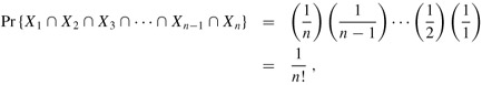
and we have shown that the probability of obtaining the identity permutation is 1/n!.
We can extend this proof to work for any permutation of priorities. Consider any fixed permutation σ = <σ(1), σ(2), ..., σ(n)> of the set {1, 2, ..., n}. Let us denote by ri the rank of the priority assigned to element A[i], where the element with the jth smallest priority has rank j. If we define Xi as the event in which element A[i] receives the σ(i)th smallest priority, or ri = σ(i), the same proof still applies. Therefore, if we calculate the probability of obtaining any particular permutation, the calculation is identical to the one above, so that the probability of obtaining this permutation is also 1/n!.
One might think that to prove that a permutation is a uniform random permutation it suffices to show that, for each element A[i], the probability that it winds up in position j is 1/n. Exercise 5.3-4 shows that this weaker condition is, in fact, insufficient.
A better method for generating a random permutation is to permute the given array in place. The procedure RANDOMIZE-IN-PLACE does so in O(n) time. In iteration i, the element A[i] is chosen randomly from among elements A[i] through A[n]. Subsequent to iteration i, A[i] is never altered.
RANDOMIZE-IN-PLACE(A)
1 n ← length[A]
2 for i ← to n
3      do swap A[i] ↔ A[RANDOM(i, n)]
We will use a loop invariant to show that procedure RANDOMIZE-IN-PLACE produces a uniform random permutation. Given a set of n elements, a k-permutation is a sequence containing k of the n elements. (See Appendix B.) There are n!/(n - k)! such possible k-permutations.
Procedure RANDOMIZE-IN-PLACE computes a uniform random permutation.
Proof We use the following loop invariant:
Just prior to the ith iteration of the for loop of lines 2-3, for each possible (i - 1)-permutation, the subarray A[1 .. i - 1] contains this (i - 1)-permutation with probability (n - i + 1)!/n!.
We need to show that this invariant is true prior to the first loop iteration, that each iteration of the loop maintains the invariant, and that the invariant provides a useful property to show correctness when the loop terminates.
Initialization: Consider the situation just before the first loop iteration, so that i = 1. The loop invariant says that for each possible 0-permutation, the sub-array A[1 .. 0] contains this 0-permutation with probability (n - i + 1)!/n! = n!/n! = 1. The subarray A[1 .. 0] is an empty subarray, and a 0-permutation has no elements. Thus, A[1 .. 0] contains any 0-permutation with probability 1, and the loop invariant holds prior to the first iteration.
Maintenance: We assume that just before the (i - 1)st iteration, each possible (i - 1)-permutation appears in the subarray A[1 .. i - 1] with probability (n - i + 1)!/n!, and we will show that after the ith iteration, each possible i-permutation appears in the subarray A[1 .. i] with probability (n - i)!/n!. Incrementing i for the next iteration will then maintain the loop invariant.
Let us examine the ith iteration. Consider a particular i-permutation, and denote the elements in it by <x1, x2, ..., xi>. This permutation consists of an (i - 1)-permutation <x1, ..., xi-1> followed by the value xi that the algorithm places in A[i]. Let E1 denote the event in which the first i - 1 iterations have created the particular (i - 1)-permutation <x1,..., xi-1> in A[1 .. i - 1]. By the loop invariant, Pr {E1} = (n - i + 1)!/n!. Let E2 be the event that ith iteration puts xi in position A[i]. The i-permutation <x1, ..., xi> is formed in A[1 .. i] precisely when both E1 and E2 occur, and so we wish to compute Pr {E2 ∩ E1}. Using equation (C.14), we have
Pr {E2 ∩ E1} = Pr{E2 | E1}Pr{E1}.
The probability Pr {E2 | E1} equals 1/(n-i + 1) because in line 3 the algorithm chooses xi randomly from the n - i + 1 values in positions A[i .. n]. Thus, we have
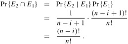
Termination: At termination, i = n + 1, and we have that the subarray A[1 .. n] is a given n-permutation with probability (n - n)!/n! = 1/n!.
Thus, RANDOMIZE-IN-PLACE produces a uniform random permutation.
A randomized algorithm is often the simplest and most efficient way to solve a problem. We shall use randomized algorithms occasionally throughout this book.
Professor Marceau objects to the loop invariant used in the proof of Lemma 5.5. He questions whether it is true prior to the first iteration. His reasoning is that one could just as easily declare that an empty subarray contains no 0-permutations. Therefore, the probability that an empty subarray contains a 0-permutation should be 0, thus invalidating the loop invariant prior to the first iteration. Rewrite the procedure RANDOMIZE-IN-PLACE so that its associated loop invariant applies to a nonempty subarray prior to the first iteration, and modify the proof of Lemma 5.5 for your procedure.
Professor Kelp decides to write a procedure that will produce at random any permutation besides the identity permutation. He proposes the following procedure:
PERMUTE-WITHOUT-IDENTITY(A)
1 n ← length[A]
2 for i ← 1 to n
3      do swap A[i] ↔ A[RANDOM(i + 1, n)]
Does this code do what Professor Kelp intends?
Suppose that instead of swapping element A[i] with a random element from the subarray A[i .. n], we swapped it with a random element from anywhere in the array:
PERMUTE-WITH-ALL(A)
1 n ← length[A]
2 for i ← 1 to n
3      do swap A[i] ↔ A[RANDOM(1, n)]
Does this code produce a uniform random permutation? Why or why not?
Professor Armstrong suggests the following procedure for generating a uniform random permutation:
PERMUTE-BY-CYCLIC(A)
1  n ← length[A]
2  offset ← RANDOM(1, n)
3  for i ← 1 to n
4       do dest ← i + offset
5          if dest > n
6             then dest ← dest -n
7          B[dest] ← A[i]
8  return B
Show that each element A[i] has a 1/n probability of winding up in any particular position in B. Then show that Professor Armstrong is mistaken by showing that the resulting permutation is not uniformly random.
|
|
< Day Day Up > |
|