5.2 Indicator random variables

In order to analyze many algorithms, including the hiring problem, we will use indicator random variables. Indicator random variables provide a convenient method for converting between probabilities and expectations. Suppose we are given a sample space S and an event A. Then the indicator random variable I {A} associated with event A is defined as

(5.1)

As a simple example, let us determine the expected number of heads that we obtain when flipping a fair coin. Our sample space is S = {H, T}, and we define a random variable Y which takes on the values H and T, each with probability 1/2. We can then define an indicator random variable X_H, associated with the coin coming up heads, which we can express as the event Y = H. This variable counts the number of heads obtained in this flip, and it is 1 if the coin comes up heads and 0 otherwise. We write

The expected number of heads obtained in one flip of the coin is simply the expected value of our indicator variable X_H:

Thus the expected number of heads obtained by one flip of a fair coin is 1/2. As the following lemma shows, the expected value of an indicator random variable associated with an event A is equal to the probability that A occurs.

Lemma 5.1

Given a sample space S and an event A in the sample space S, let X_A = I{A}. Then E[X_A] = Pr{A}.

Proof By the definition of an indicator random variable from equation 1) and the definition of expected value, we have

E[XA]	=	E[I{A}]
	=	1 · Pr{A} + 0 · Pr{}
	=	Pr{A},

where denotes S - A, the complement of A.

Although indicator random variables may seem cumbersome for an application such as counting the expected number of heads on a flip of a single coin, they are useful for analyzing situations in which we perform repeated random trials. For example, indicator random variables give us a simple way to arrive at the result of equation (C.36). In this equation, we compute the number of heads in n coin flips by considering separately the probability of obtaining 0 heads, 1 heads, 2 heads, etc. However, the simpler method proposed in equation (C.37) actually implicitly uses indicator random variables. Making this argument more explicit, we can let X_i be the indicator random variable associated with the event in which the ith flip comes up heads. Letting Y_i be the random variable denoting the outcome of the ith flip, we have that X_i = I{Y_i = H}. Let X be the random variable denoting the total number of heads in the n coin flips, so that

We wish to compute the expected number of heads, so we take the expectation of both sides of the above equation to obtain

The left side of the above equation is the expectation of the sum of n random variables. By Lemma 5.1, we can easily compute the expectation of each of the random variables. By equation (C.20)-linearity of expectation-it is easy to compute the expectation of the sum: it equals the sum of the expectations of the n random variables. Linearity of expectation makes the use of indicator random variables a powerful analytical technique; it applies even when there is dependence among the random variables. We now can easily compute the expected number of heads:

Thus, compared to the method used in equation (C.36), indicator random variables greatly simplify the calculation. We shall use indicator random variables throughout this book.

Analysis of the hiring problem using indicator random variables

Returning to the hiring problem, we now wish to compute the expected number of times that we hire a new office assistant. In order to use a probabilistic analysis, we assume that the candidates arrive in a random order, as discussed in the previous section. (We shall see in Section 5.3 how to remove this assumption.) Let X be the random variable whose value equals the number of times we hire a new office assistant. We could then apply the definition of expected value from equation (C.19) to obtain

but this calculation would be cumbersome. We shall instead use indicator random variables to greatly simplify the calculation.

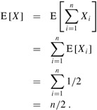
To use indicator random variables, instead of computing E[X] by defining one variable associated with the number of times we hire a new office assistant, we define n variables related to whether or not each particular candidate is hired. In particular, we let X_i be the indicator random variable associated with the event in which the ith candidate is hired. Thus,

(5.2)

and

(5.3)

By Lemma 5.1, we have that

E[X_i] = Pr {candidate i is hired},

and we must therefore compute the probability that lines 5-6 of HIRE-ASSISTANT are executed.

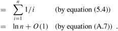
Candidate i is hired, in line 5, exactly when candidate i is better than each of candidates 1 through i - 1. Because we have assumed that the candidates arrive in a random order, the first i candidates have appeared in a random order. Any one of these first i candidates is equally likely to be the best-qualified so far. Candidate i has a probability of 1/i of being better qualified than candidates 1 through i - 1 and thus a probability of 1/i of being hired. By Lemma 5.1, we conclude that

(5.4)

Now we can compute E[X]:

(5.5)

(5.6)

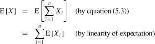Even though we interview n people, we only actually hire approximately ln n of them, on average. We summarize this result in the following lemma.

Lemma 5.2

Assuming that the candidates are presented in a random order, algorithm HIRE-ASSISTANT has a total hiring cost of O(c_h ln n).

Proof The bound follows immediately from our definition of the hiring cost and equation (5.6).

The expected interview cost is a significant improvement over the worst-case hiring cost of O(nc_h).

Exercises 5.2-1

In HIRE-ASSISTANT, assuming that the candidates are presented in a random order, what is the probability that you will hire exactly one time? What is the probability that you will hire exactly n times?

Exercises 5.2-2

In HIRE-ASSISTANT, assuming that the candidates are presented in a random order, what is the probability that you will hire exactly twice?

Exercises 5.2-3

Use indicator random variables to compute the expected value of the sum of n dice.

Exercises 5.2-4

Use indicator random variables to solve the following problem, which is known as the hat-check problem. Each of n customers gives a hat to a hat-check person at a restaurant. The hat-check person gives the hats back to the customers in a random order. What is the expected number of customers that get back their own hat?

Exercises 5.2-5

Let A[1 .. n] be an array of n distinct numbers. If i < j and A[i] > A[j], then the pair (i, j) is called an inversion of A. (See Problem 2-4 for more on inversions.) Suppose that each element of A is chosen randomly, independently, and uniformly from the range 1 through n. Use indicator random variables to compute the expected number of inversions.