The structure of a shortest path

We start by characterizing the structure of an optimal solution. For the all-pairs shortest-paths problem on a graph G = (V, E), we have proven (Lemma 24.1) that all subpaths of a shortest path are shortest paths. Suppose that the graph is represented by an adjacency matrix W = (w_ij). Consider a shortest path p from vertex i to vertex j, and suppose that p contains at most m edges. Assuming that there are no negative-weight cycles, m is finite. If i = j, then p has weight 0 and no edges. If vertices i and j are distinct, then we decompose path p into , where path p′ now contains at most m - 1 edges. By Lemma 24.1, p′ is a shortest path from i to k, and so δ(i, j) = δ(i, k) + w_kj.

A recursive solution to the all-pairs shortest-paths problem

Now, let be the minimum weight of any path from vertex i to vertex j that contains at most m edges. When m = 0, there is a shortest path from i to j with no edges if and only if i = j. Thus,

For m ≥ 1, we compute as the minimum of (the weight of the shortest path from i to j consisting of at most m - 1 edges) and the minimum weight of any path from i to j consisting of at most m edges, obtained by looking at all possible predecessors k of j. Thus, we recursively define

(25.2)

The latter equality follows since w_jj = 0 for all j.

What are the actual shortest-path weights δ(i, j)? If the graph contains no negative-weight cycles, then for every pair of vertices i and j for which δ(i, j) < ∞, there is a shortest path from i to j that is simple and thus contains at most n - 1 edges. A path from vertex i to vertex j with more than n - 1 edges cannot have lower weight than a shortest path from i to j. The actual shortest-path weights are therefore given by

(25.3)

Computing the shortest-path weights bottom up

Taking as our input the matrix W = (w_ij), we now compute a series of matrices L⁽¹⁾, L⁽²⁾,..., L^(n-1), where for m = 1, 2,..., n - 1, we have . The final matrix L^(n-1) contains the actual shortest-path weights. Observe that for all vertices i, j ∈ V , and so L⁽¹⁾ = W.

The heart of the algorithm is the following procedure, which, given matrices L^(m-1) and W, returns the matrix L^(m). That is, it extends the shortest paths computed so far by one more edge.

EXTEND-SHORTEST-PATHS(L, W)
1  n ← rows[L]
2  let  be an n × n matrix
3  for i ← 1 to n
4      do for j ← to n
5            do 
6              for k ← 1 to n
7                  do 
8  return L′

The procedure computes a matrix , which it returns at the end. It does so by computing equation (25.2) for all i and j, using L for L^(m-1) and L′ for L^(m). (It is written without the superscripts to make its input and output matrices independent of m.) Its running time is Θ(n³) due to the three nested for loops.

Now we can see the relation to matrix multiplication. Suppose we wish to compute the matrix product C = A · B of two n × n matrices A and B. Then, for i, j = 1, 2,..., n, we compute

(25.4)

Observe that if we make the substitutions

in equation (25.2), we obtain equation (25.4). Thus, if we make these changes to EXTEND-SHORTEST-PATHS and also replace ∞ (the identity for min) by 0 (the identity for +), we obtain the straightforward Θ(n³)-time procedure for matrix multiplication:

MATRIX-MULTIPLY(A, B)
1  n ← rows[A]
2  let C be an n × n matrix
3  for i ← 1 to n
4      do for j ← 1 to n
5           do cij ← 0
6              for k ← 1 to n
7                do cij ← cij + aik · bkj
8  return C

Returning to the all-pairs shortest-paths problem, we compute the shortest-path weights by extending shortest paths edge by edge. Letting A · B denote the matrix "product" returned by EXTEND-SHORTEST-PATHS(A, B), we compute the sequence of n - 1 matrices

As we argued above, the matrix L^(n-1) = W^n-1 contains the shortest-path weights. The following procedure computes this sequence in Θ(n⁴) time.

SLOW-ALL-PAIRS-SHORTEST-PATHS(W)
1  n ← rows[W]
2  L(1) W
3  for m ← 2 to n - 1
4      do L(m) ← EXTEND-SHORTEST-PATHS(L(m-1), W)
5  return L(n-1)

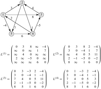
Figure 25.1 shows a graph and the matrices L^(m) computed by the procedure SLOW-ALL-PAIRS-SHORTEST-PATHS.

Figure 25.1: A directed graph and the sequence of matrices L^(m) computed by SLOW-ALL-PAIRS-SHORTEST-PATHS. The reader may verify that L⁽⁵⁾ = L⁽⁴⁾ · W is equal to L⁽⁴⁾, and thus L^(m) = L⁽⁴⁾ for all m ≥ 4.

Improving the running time

Our goal, however, is not to compute all the L^(m) matrices: we are interested only in matrix L^(n-1). Recall that in the absence of negative-weight cycles, equation (25.3) implies L^(m) = L^(n-1) for all integers m ≥ n - 1. Just as traditional matrix multiplication is associative, so is matrix multiplication defined by the EXTEND-SHORTEST-PATHS procedure (see Exercise 25.1-4). Therefore, we can compute L^(n-1) with only ⌈lg(n - 1)⌉ matrix products by computing the sequence

Since 2^{⌈lg(n-1)⌉} ≥ n - 1, the final product is equal to L^(n-1).

The following procedure computes the above sequence of matrices by using this technique of repeated squaring.

FASTER-ALL-PAIRS-SHORTEST-PATHS(W)
1  n ← rows[W]
2  L(1) ← W
3  m ← 1
4  while m < n - 1
5      do L(2m) ← EXTEND-SHORTEST-PATHS(L(m), L(m))
6         m ← 2m
7  return L(m)

In each iteration of the while loop of lines 4-6, we compute L^(2m) = (L^(m))², starting with m = 1. At the end of each iteration, we double the value of m. The final iteration computes L^(n-1) by actually computing L^(2m) for some n - 1 ≤ 2m < 2n - 2. By equation (25.3), L^(2m) = L^(n-1). The next time the test in line 4 is performed, m has been doubled, so now m ≥ n - 1, the test fails, and the procedure returns the last matrix it computed.

The running time of FASTER-ALL-PAIRS-SHORTEST-PATHS is Θ(n³ lg n) since each of the ⌈lg(n - 1)⌉ matrix products takes Θ(n³) time. Observe that the code is tight, containing no elaborate data structures, and the constant hidden in the Θ-notation is therefore small.

Exercises 25.1-1

Run SLOW-ALL-PAIRS-SHORTEST-PATHS on the weighted, directed graph of Figure 25.2, showing the matrices that result for each iteration of the loop. Then do the same for FASTER-ALL-PAIRS-SHORTEST-PATHS.

Figure 25.2: A weighted, directed graph for use in Exercises 25.1-1, 25.2-1, and 25.3-1.

Exercises 25.1-2

Why do we require that w_ii = 0 for all 1 ≤ i ≤ n?

Exercises 25.1-3

What does the matrix

used in the shortest-paths algorithms correspond to in regular matrix multiplication?

Exercises 25.1-4

Show that matrix multiplication defined by EXTEND-SHORTEST-PATHS is associative.

Exercises 25.1-5

Show how to express the single-source shortest-paths problem as a product of matrices and a vector. Describe how evaluating this product corresponds to a Bellman-Ford-like algorithm (see Section 24.1).

Exercises 25.1-6

Suppose we also wish to compute the vertices on shortest paths in the algorithms of this section. Show how to compute the predecessor matrix Π from the completed matrix L of shortest-path weights in O(n³) time.

Exercises 25.1-7

The vertices on shortest paths can also be computed at the same time as the shortest-path weights. Let us define to be the predecessor of vertex j on any minimum-weight path from i to j that contains at most m edges. Modify EXTEND-SHORTEST-PATHS and SLOW-ALL-PAIRS-SHORTEST-PATHS to compute the matrices Π⁽¹⁾, Π⁽²⁾,..., Π^(n-1) as the matrices L⁽¹⁾, L⁽²⁾,..., L^(n-1) are computed.

Exercises 25.1-8

The FASTER-ALL-PAIRS-SHORTEST-PATHS procedure, as written, requires us to store ⌈lg(n - 1)⌉ matrices, each with n² elements, for a total space requirement of Θ(n² lg n). Modify the procedure to require only Θ(n²) space by using only two n × n matrices.

Exercises 25.1-9

Modify FASTER-ALL-PAIRS-SHORTEST-PATHS so that it can detect the presence of a negative-weight cycle.

Exercises 25.1-10

Give an efficient algorithm to find the length (number of edges) of a minimum-length negative-weight cycle in a graph.