The structure of a shortest path

In the Floyd-Warshall algorithm, we use a different characterization of the structure of a shortest path than we used in the matrix-multiplication-based all-pairs algorithms. The algorithm considers the "intermediate" vertices of a shortest path, where an intermediate vertex of a simple path p = <v₁, v₂,..., v_l> is any vertex of p other than v₁ or v_l, that is, any vertex in the set {v₂, v₃,..., v_l-1}.

The Floyd-Warshall algorithm is based on the following observation. Under our assumption that the vertices of G are V = {1, 2,..., n}, let us consider a subset {1, 2,..., k} of vertices for some k. For any pair of vertices i, j ∈ V, consider all paths from i to j whose intermediate vertices are all drawn from {1, 2,..., k}, and let p be a minimum-weight path from among them. (Path p is simple.) The Floyd-Warshall algorithm exploits a relationship between path p and shortest paths from i to j with all intermediate vertices in the set {1, 2,..., k - 1}. The relationship depends on whether or not k is an intermediate vertex of path p.

• If k is not an intermediate vertex of path p, then all intermediate vertices of path p are in the set {1, 2,..., k - 1}. Thus, a shortest path from vertex i to vertex j with all intermediate vertices in the set {1, 2,..., k - 1} is also a shortest path from i to j with all intermediate vertices in the set {1, 2,..., k}.

• If k is an intermediate vertex of path p, then we break p down into as shown in Figure 25.3. By Lemma 24.1, p₁ is a shortest path from i to k with all intermediate vertices in the set {1, 2,..., k}. Because vertex k is not an intermediate vertex of path p₁, we see that p₁ is a shortest path from i to k with all intermediate vertices in the set {1, 2,..., k - 1}. Similarly, p₂ is a shortest path from vertex k to vertex j with all intermediate vertices in the set {1, 2,..., k - 1}.

  
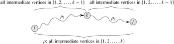
  Figure 25.3: Path p is a shortest path from vertex i to vertex j, and k is the highest-numbered intermediate vertex of p. Path p₁, the portion of path p from vertex i to vertex k, has all intermediate vertices in the set {1, 2,..., k - 1}. The same holds for path p₂ from vertex k to vertex j.

A recursive solution to the all-pairs shortest-paths problem

Based on the above observations, we define a recursive formulation of shortest-path estimates that is different from the one in Section 25.1. Let be the weight of a shortest path from vertex i to vertex j for which all intermediate vertices are in the set {1, 2,..., k}. When k = 0, a path from vertex i to vertex j with no intermediate vertex numbered higher than 0 has no intermediate vertices at all. Such a path has at most one edge, and hence . A recursive definition following the above discussion is given by

(25.5)

Because for any path, all intermediate vertices are in the set {1, 2,..., n}, the matrix gives the final answer: for all i, j ∈ V.

Computing the shortest-path weights bottom up

Based on recurrence (25.5), the following bottom-up procedure can be used to compute the values in order of increasing values of k. Its input is an n × n matrix W defined as in equation (25.1). The procedure returns the matrix D⁽ⁿ⁾ of shortest-path weights.

FLOYD-WARSHALL(W)
1  n ← rows[W]
2  D(0) ← W
3  for k ← 1 to n
4       do for i ← 1 to n
5              do for j ← 1 to n
6                     do 
7  return D(n)

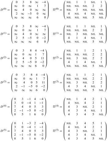
Figure 25.4 shows the matrices D^(k) computed by the Floyd-Warshall algorithm for the graph in Figure 25.1.

Figure 25.4: The sequence of matrices D^(k) and Π^(k) computed by the Floyd-Warshall algorithm for the graph in Figure 25.1.

The running time of the Floyd-Warshall algorithm is determined by the triply nested for loops of lines 3-6. Because each execution of line 6 takes O(1) time, the algorithm runs in time Θ(n³). As in the final algorithm in Section 25.1, the code is tight, with no elaborate data structures, and so the constant hidden in the Θ-notation is small. Thus, the Floyd-Warshall algorithm is quite practical for even moderate-sized input graphs.

Constructing a shortest path

There are a variety of different methods for constructing shortest paths in the Floyd-Warshall algorithm. One way is to compute the matrix D of shortest-path weights and then construct the predecessor matrix Π from the D matrix. This method can be implemented to run in O(n³) time (Exercise 25.1-6). Given the predecessor matrix Π, the PRINT-ALL-PAIRS-SHORTEST-PATH procedure can be used to print the vertices on a given shortest path.

We can compute the predecessor matrix Π "on-line" just as the Floyd-Warshall algorithm computes the matrices D^(k). Specifically, we compute a sequence of matrices Π⁽⁰⁾, Π⁽¹⁾,..., Π⁽ⁿ⁾, where Π = Π⁽ⁿ⁾ and is defined to be the predecessor of vertex j on a shortest path from vertex i with all intermediate vertices in the set {1, 2,..., k}.

We can give a recursive formulation of . When k = 0, a shortest path from i to j has no intermediate vertices at all. Thus,

(25.6)

For k ≥ 1, if we take the path , where k ≠ j, then the predecessor of j we choose is the same as the predecessor of j we chose on a shortest path from k with all intermediate vertices in the set {1, 2,...,k - 1}. Otherwise, we choose the same predecessor of j that we chose on a shortest path from i with all intermediate vertices in the set {1, 2,..., k - 1}. Formally, for k ≥ 1,

(25.7)

We leave the incorporation of the Π^(k) matrix computations into the FLOYD-WARSHALL procedure as Exercise 25.2-3. Figure 25.4 shows the sequence of Π^(k) matrices that the resulting algorithm computes for the graph of Figure 25.1.The exercise also asks for the more difficult task of proving that the predecessor subgraph G_π,i is a shortest-paths tree with root i. Yet another way to reconstruct shortest paths is given as Exercise 25.2-7.

Transitive closure of a directed graph

Given a directed graph G = (V, E) with vertex set V = {1, 2,...,n}, we may wish to find out whether there is a path in G from i to j for all vertex pairs i, j ∈ V. The transitive closure of G is defined as the graph G* = (V, E*), where E*= {(i, j) : there is a path from vertex i to vertex j in G}.

One way to compute the transitive closure of a graph in Θ(n³) time is to assign a weight of 1 to each edge of E and run the Floyd-Warshall algorithm. If there is a path from vertex i to vertex j, we get d_ij < n. Otherwise, we get d_ij = ∞.

There is another, similar way to compute the transitive closure of G in Θ(n³) time that can save time and space in practice. This method involves substitution of the logical operations ∨ (logical OR) and ∧ (logical AND) for the arithmetic operations min and + in the Floyd-Warshall algorithm. For i, j, k = 1, 2,...,n, we define to be 1 if there exists a path in graph G from vertex i to vertex j with all intermediate vertices in the set {1, 2,..., k}, and 0 otherwise. We construct the transitive closure G* = (V, E*) by putting edge (i, j) into E* if and only if . A recursive definition of , analogous to recurrence (25.5), is

and for k ≥ 1,

(25.8)

As in the Floyd-Warshall algorithm, we compute the matrices in order of increasing k.

TRANSITIVE-CLOSURE(G)
 1  n ← |V[G]|
 2  for i ← 1 to n
 3       do for j ← 1 to n
 4              do if i = j or (i, j) ∈ E[G]
 5                    then 
 6                    else 
 7  for k ← 1 to n
 8       do for i ← 1 to n
 9              do for j ← 1 to n
10                     do 
11  return T(n)

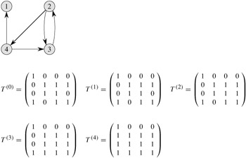
Figure 25.5 shows the matrices T^(k) computed by the TRANSITIVE-CLOSURE procedure on a sample graph. The TRANSITIVE-CLOSURE procedure, like the Floyd-Warshall algorithm, runs in Θ(n³) time. On some computers, though, logical operations on single-bit values execute faster than arithmetic operations on integer words of data. Moreover, because the direct transitive-closure algorithm uses only boolean values rather than integer values, its space requirement is less than the Floyd-Warshall algorithm's by a factor corresponding to the size of a word of computer storage.

Figure 25.5: A directed graph and the matrices T^(k) computed by the transitive-closure algorithm.

Exercises 25.2-1

Run the Floyd-Warshall algorithm on the weighted, directed graph of Figure 25.2. Show the matrix D^(k) that results for each iteration of the outer loop.

Exercises 25.2-2

Show how to compute the transitive closure using the technique of Section 25.1.

Exercises 25.2-3

Modify the FLOYD-WARSHALL procedure to include computation of the Π^(k) matrices according to equations (25.6) and (25.7). Prove rigorously that for all i ∈ V , the predecessor subgraph G_π,i is a shortest-paths tree with root i. (Hint: To show that G_π,i is acyclic, first show that implies , according to the definition of . Then, adapt the proof of Lemma 24.16.)

Exercises 25.2-4

As it appears above, the Floyd-Warshall algorithm requires Θ(n³) space, since we compute for i, j, k = 1, 2,...,n. Show that the following procedure, which simply drops all the superscripts, is correct, and thus only Θ(n²) space is required.

FLOYD-WARSHALL′ (W)
1  n ← rows[W]
2  D ← W
3  for k ← 1 to n
4       do for i ← 1 to n
5              do for j ← 1 to n
6                     do dij ← min (dij, dik + dkj)
7  return D

Exercises 25.2-5

Suppose that we modify the way in which equality is handled in equation (25.7):

Is this alternative definition of the predecessor matrix Π correct?

Exercises 25.2-6

How can the output of the Floyd-Warshall algorithm be used to detect the presence of a negative-weight cycle?

Exercises 25.2-7

Another way to reconstruct shortest paths in the Floyd-Warshall algorithm uses values for i, j, k = 1, 2,..., n, where is the highest-numbered intermediate vertex of a shortest path from i to j in which all intermediate vertices are in the set {1, 2,..., k}. Give a recursive formulation for , modify the FLOYD-WARSHALL procedure to compute the values, and rewrite the PRINT-ALL-PAIRS-SHORTEST-PATH procedure to take the matrix as an input. How is the matrix Θ like the s table in the matrix-chain multiplication problem of Section 15.2?

Exercises 25.2-8

Give an O(V E)-time algorithm for computing the transitive closure of a directed graph G = (V, E).

Exercises 25.2-9

Suppose that the transitive closure of a directed acyclic graph can be computed in f(|V|,|E|) time, where f is a monotonically increasing function of |V| and |E|. Show that the time to compute the transitive closure G* = (V, E*) of a general directed graph G = (V, E) is f(|V|,|E|) + O(V + E*).