|
|
< Day Day Up > |
|
Solving a set of simultaneous linear equations is a fundamental problem that occurs in diverse applications. A linear system can be expressed as a matrix equation in which each matrix or vector element belongs to a field, typically the real numbers R. This section discusses how to solve a system of linear equations using a method called LUP decomposition.
We start with a set of linear equations in n unknowns x1, x2, . . . , xn:
A set of values for x1, x2, . . . , xn that satisfy all of the equations (28.16) simultaneously is said to be a solution to these equations. In this section, we treat only the case in which there are exactly n equations in n unknowns.
We can conveniently rewrite equations (28.16) as the matrix-vector equation

or, equivalently, letting A = (aij), x = (xi), and b = (bi), as
If A is nonsingular, it possesses an inverse A-1, and
| (28.18) |
is the solution vector. We can prove that x is the unique solution to equation (28.17) as follows. If there are two solutions, x and x′, then Ax = Ax′ = b and
|
x |
= |
(A-1A)x |
|
= |
A-1(Ax) |
|
|
= |
A-1(Ax′) |
|
|
= |
(A-1A)x′ |
|
|
= |
x′. |
In this section, we shall be concerned predominantly with the case in which A is nonsingular or, equivalently (by Theorem 28.1), the rank of A is equal to the number n of unknowns. There are other possibilities, however, which merit a brief discussion. If the number of equations is less than the number n of unknowns-or, more generally, if the rank of A is less than n-then the system is underdetermined. An underdetermined system typically has infinitely many solutions, although it may have no solutions at all if the equations are inconsistent. If the number of equations exceeds the number n of unknowns, the system is overdetermined, and there may not exist any solutions. Finding good approximate solutions to overdetermined systems of linear equations is an important problem that is addressed in Section 28.5.
Let us return to our problem of solving the system Ax = b of n equations in n unknowns. One approach is to compute A-1 and then multiply both sides by A-1, yielding A-1 Ax = A-1b, or x = A-1b. This approach suffers in practice from numerical instability. There is, fortunately, another approach-LUP decomposition-that is numerically stable and has the further advantage of being faster in practice.
The idea behind LUP decomposition is to find three n × n matrices L, U, and P such that
where
L is a unit lower-triangular matrix,
U is an upper-triangular matrix, and
P is a permutation matrix.
We call matrices L, U , and P satisfying equation (28.19) an LUP decomposition of the matrix A. We shall show that every nonsingular matrix A possesses such a decomposition.
The advantage of computing an LUP decomposition for the matrix A is that linear systems can be solved more readily when they are triangular, as is the case for both matrices L and U . Having found an LUP decomposition for A, we can solve the equation (28.17) Ax = b by solving only triangular linear systems, as follows. Multiplying both sides of Ax = b by P yields the equivalent equation P Ax = Pb, which by Exercise 28.1-5 amounts to permuting the equations (28.16).Using our decomposition (28.19), we obtain
LU x = Pb.
We can now solve this equation by solving two triangular linear systems. Let us define y = U x, where x is the desired solution vector. First, we solve the lower-triangular system
for the unknown vector y by a method called "forward substitution." Having solved for y, we then solve the upper-triangular system
for the unknown x by a method called "back substitution." The vector x is our solution to Ax = b, since the permutation matrix P is invertible (Exercise 28.1-5):
|
Ax |
= |
P-1LU x |
|
= |
P-1Ly |
|
|
= |
P-1Pb |
|
|
= |
b. |
Our next step is to show how forward and back substitution work and then attack the problem of computing the LUP decomposition itself.
Forward substitution can solve the lower-triangular system (28.20) in Θ(n2) time, given L, P, and b. For convenience, we represent the permutation P compactly by an array π[1 ‥ n]. For i = 1, 2, . . . , n, the entry π[i] indicates that Pi, π[i] = 1 and Pij = 0 for j ≠ π[i]. Thus, P A has aπ[i], j in row i and column j, and Pb has bπ[i] as its ith element. Since L is unit lower-triangular, equation (28.20) can be rewritten as
|
y1 |
= |
bπ[1], |
|
l21y1 + y2 |
= |
bπ[2], |
|
l31y1 + l32y2 + y3 |
= |
bπ[3], |
|
⋮ | ||
|
ln1y1 + ln2y2 + ln3y3 + · · · + yn |
= |
bπ[n]. |
We can solve for y1 directly, since the first equation tells us that y1 = bπ[1]. Having solved for y1, we can substitute it into the second equation, yielding
y2 = bπ[2] - l21y1.
Now, we can substitute both y1 and y2 into the third equation, obtaining
y3 = bπ[3] - (l31y1 + l32y2).
In general, we substitute y1, y2, . . . , yi-1 "forward" into the ith equation to solve for yi:
Back substitution is similar to forward substitution. Given U and y, we solve the nth equation first and work backward to the first equation. Like forward substitution, this process runs in Θ(n2) time. Since U is upper-triangular, we can rewrite the system (28.21) as
|
u11x1 + u12x2 + · · · + u1, n-2xn-2 + u1, n-1xn-1 + u1nxn |
= |
y1, |
|
u22x2 + · · · + u2, n-2xn-2 + u2, n-1xn-1 + u2nxn |
= |
y2, |
|
⋮ | ||
|
un-2, n-2xn-2 + un-2, n-1xn-1 + un-2, nxn |
= |
yn-2, |
|
un-1,n-1xn-1 + un-1, nxn |
= |
yn-1, |
|
un,nxn |
= |
yn. |
Thus, we can solve for xn, xn-1, . . . , x1 successively as follows:
|
xn |
= |
yn/un,n, |
|
xn-1 |
= |
(yn-1 - un-1,nxn)/un-1,n-1, |
|
xn-2 |
= |
(yn-2 - (un-2,n-1xn-1 + un-2,nxn))/un-2,n-2, |
|
⋮ |
or, in general,
Given P, L, U , and b, the procedure LUP-SOLVE solves for x by combining forward and back substitution. The pseudocode assumes that the dimension n appears in the attribute rows[L] and that the permutation matrix P is represented by the array π.
LUP-SOLVE(L, U, π, b) 1 n ← rows[L] 2 for i ← 1 to n 3 do4 for i ← n downto 1 5 do
6 return x
Procedure LUP-SOLVE solves for y using forward substitution in lines 2-3, and then it solves for x using backward substitution in lines 4-5. Since there is an implicit loop in the summations within each of the for loops, the running time is Θ(n2).
As an example of these methods, consider the system of linear equations defined by

where

and we wish to solve for the unknown x. The LUP decomposition is

(The reader can verify that P A = LU.) Using forward substitution, we solve Ly = Pb for y:

obtaining

by computing first y1, then y2, and finally y3. Using back substitution, we solve U x = y for x:

thereby obtaining the desired answer

by computing first x3, then x2, and finally x1.
We have now shown that if an LUP decomposition can be computed for a nonsingular matrix A, forward and back substitution can be used to solve the system Ax = b of linear equations. It remains to show how an LUP decomposition for A can be found efficiently. We start with the case in which A is an n × n nonsingular matrix and P is absent (or, equivalently, P = In). In this case, we must find a factorization A = LU . We call the two matrices L and U an LU decomposition of A.
The process by which we perform LU decomposition is called Gaussian elimination. We start by subtracting multiples of the first equation from the other equations so that the first variable is removed from those equations. Then, we subtract multiples of the second equation from the third and subsequent equations so that now the first and second variables are removed from them. We continue this process until the system that is left has an upper-triangular form-in fact, it is the matrix U. The matrix L is made up of the row multipliers that cause variables to be eliminated.
Our algorithm to implement this strategy is recursive. We wish to construct an LU decomposition for an n × n nonsingular matrix A. If n = 1, then we're done, since we can choose L = I1 and U = A. For n > 1, we break A into four parts:

where v is a size-(n - 1) column vector, wT is a size-(n - 1) row vector, and A′ is an (n - 1) × (n - 1) matrix. Then, using matrix algebra (verify the equations by simply multiplying through), we can factor A as
| (28.22) |  |
The 0's in the first and second matrices of the factorization are row and column vectors, respectively, of size n - 1. The term vwT/a11, formed by taking the outer product of v and w and dividing each element of the result by a11, is an (n - 1) × (n - 1) matrix, which conforms in size to the matrix A′ from which it is subtracted. The resulting (n - 1) × (n - 1) matrix
is called the Schur complement of A with respect to a11.
We claim that if A is nonsingular, then the Schur complement is nonsingular, too. Why? Suppose that the Schur complement, which is (n - 1) × (n - 1), is singular. Then by Theorem 28.1, it has row rank strictly less than n - 1. Because the bottom n - 1 entries in the first column of the matrix
are all 0, the bottom n - 1 rows of this matrix must have row rank strictly less than n - 1. The row rank of the entire matrix, therefore, is strictly less than n. Applying Exercise 28.1-10 to equation (28.22), A has rank strictly less than n, and from Theorem 28.1 we derive the contradiction that A is singular.
Because the Schur complement is nonsingular, we can now recursively find an LU decomposition of it. Let us say that
A′ - vwT/a11 = L′U′,
where L′ is unit lower-triangular and U′ is upper-triangular. Then, using matrix algebra, we have

thereby providing our LU decomposition. (Note that because L′ is unit lower-triangular, so is L, and because U′ is upper-triangular, so is U.)
Of course, if a11 = 0, this method doesn't work, because it divides by 0. It also doesn't work if the upper leftmost entry of the Schur complement A′ - vwT/a11 is 0, since we divide by it in the next step of the recursion. The elements by which we divide during LU decomposition are called pivots, and they occupy the diagonal elements of the matrix U. The reason we include a permutation matrix P during LUP decomposition is that it allows us to avoid dividing by zero elements. Using permutations to avoid division by 0 (or by small numbers) is called pivoting.
An important class of matrices for which LU decomposition always works correctly is the class of symmetric positive-definite matrices. Such matrices require no pivoting, and thus the recursive strategy outlined above can be employed without fear of dividing by 0. We shall prove this result, as well as several others, in Section 28.5.
Our code for LU decomposition of a matrix A follows the recursive strategy, except that an iteration loop replaces the recursion. (This transformation is a standard optimization for a "tail-recursive" procedure-one whose last operation is a recursive call to itself.) It assumes that the dimension of A is kept in the attribute rows[A]. Since we know that the output matrix U has 0's below the diagonal, and since LUP-SOLVE does not look at these entries, the code does not bother to fill them in. Likewise, because the output matrix L has 1's on its diagonal and 0's above the diagonal, these entries are not filled in either. Thus, the code computes only the "significant" entries of L and U.
LU-DECOMPOSITION(A) 1 n ← rows[A] 2 for k ← 1 to n 3 do ukk ← akk 4 for i ← k + 1 to n 5 do lik ← aik/ukk ▹lik holds vi 6 uki ← aki ▹uki holds7 for i ← k + 1 to n 8 do for j ← k + 1 to n 9 do aij ← aij - likukj 10 return L and U
The outer for loop beginning in line 2 iterates once for each recursive step. Within this loop, the pivot is determined to be ukk = akk in line 3. Within the for loop in lines 4-6 (which does not execute when k = n), the v and wT vectors are used to update L and U . The elements of the v vector are determined in line 5, where vi is stored in lik, and the elements of the wT vector are determined in line 6, where ![]() is stored in uki . Finally, the elements of the Schur complement are computed in lines 7-9 and stored back in the matrix A. (We don't need to divide by akk in line 9 because we already did so when we computed lik in line 5.) Because line 9 is triply nested, LU-DECOMPOSITION runs in time Θ(n3).
is stored in uki . Finally, the elements of the Schur complement are computed in lines 7-9 and stored back in the matrix A. (We don't need to divide by akk in line 9 because we already did so when we computed lik in line 5.) Because line 9 is triply nested, LU-DECOMPOSITION runs in time Θ(n3).
Figure 28.1 illustrates the operation of LU-DECOMPOSITION. It shows a standard optimization of the procedure in which the significant elements of L and U are stored "in place" in the matrix A. That is, we can set up a correspondence between each element aij and either lij (if i > j) or uij (if i ≤ j) and update the matrix A so that it holds both L and U when the procedure terminates. The pseudocode for this optimization is obtained from the above pseudocode merely by replacing each reference to l or u by a; it is not difficult to verify that this transformation preserves correctness.
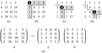
Generally, in solving a system of linear equations Ax = b, we must pivot on off-diagonal elements of A to avoid dividing by 0. Not only is division by 0 undesirable, so is division by any small value, even if A is nonsingular, because numerical instabilities can result in the computation. We therefore try to pivot on a large value.
The mathematics behind LUP decomposition is similar to that of LU decomposition. Recall that we are given an n × n nonsingular matrix A and wish to find a permutation matrix P, a unit lower-triangular matrix L, and an upper-triangular matrix U such that P A = LU . Before we partition the matrix A, as we did for LU decomposition, we move a nonzero element, say ak1, from somewhere in the first column to the (1, 1) position of the matrix. (If the first column contains only 0's, then A is singular, because its determinant is 0, by Theorems 28.4 and 28.5.) In order to preserve the set of equations, we exchange row 1 with row k, which is equivalent to multiplying A by a permutation matrix Q on the left (Exercise 28.1-5). Thus, we can write Q A as
where v = (a21, a31, . . . , an1)T, except that a11 replaces ak1; wT = (ak2, ak3, . . . , akn); and A′ is an (n - 1) × (n - 1) matrix. Since ak1 ≠ 0, we can now perform much the same linear algebra as for LU decomposition, but now guaranteeing that we do not divide by 0:

As we saw for LU decomposition, if A is nonsingular, then the Schur complement A′ - vwT/ak1 is nonsingular, too. Therefore, we can inductively find an LUP decomposition for it, with unit lower-triangular matrix L′, upper-triangular matrix U′, and permutation matrix P′, such that
P′(A′ - vwT/ak1) = L′U′.
Define
which is a permutation matrix, since it is the product of two permutation matrices (Exercise 28.1-5). We now have


yielding the LUP decomposition. Because L′ is unit lower-triangular, so is L, and because U′ is upper-triangular, so is U.
Notice that in this derivation, unlike the one for LU decomposition, both the column vector v/ak1 and the Schur complement A′ - vwT/ak1 must be multiplied by the permutation matrix P′.
Like LU-DECOMPOSITION, our pseudocode for LUP decomposition replaces the recursion with an iteration loop. As an improvement over a direct implementation of the recursion, we dynamically maintain the permutation matrix P as an array π, where π[i] = j means that the ith row of P contains a 1 in column j. We also implement the code to compute L and U "in place" in the matrix A. Thus, when the procedure terminates,
LUP-DECOMPOSITION(A)
 1 n ← rows[A]
 2 for i ← 1 to n
 3      do π[i] ← i
 4 for k ← 1 to n
 5      do p ← 0
 6         for i ← k to n
 7             do if |aik| > p
 8                   then p ← |aik|
 9                        k' ← i
10         if p = 0
11            then error "singular matrix"
12         exchange π[k] ↔ π[k']
13         for i ← 1 to n
14              do exchange aki ↔ ak'i
15         for i ← k + 1 to n
16              do aik ← aik/akk
17                 for j ← k + 1 to n
18                     do aij ← aij - aikakj
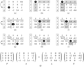
Figure 28.2 illustrates how LUP-DECOMPOSITION factors a matrix. The array π is initialized by lines 2-3 to represent the identity permutation. The outer for loop beginning in line 4 implements the recursion. Each time through the outer loop, lines 5-9 determine the element ak'k with largest absolute value of those in the current first column (column k) of the (n - k + 1) × (n - k + 1) matrix whose LU decomposition must be found. If all elements in the current first column are zero, lines 10-11 report that the matrix is singular. To pivot, we exchange π[k'] with π[k] in line 12 and exchange the kth and k'th rows of A in lines 13-14, thereby making the pivot element akk. (The entire rows are swapped because in the derivation of the method above, not only is A′ - vwT/ak1 multiplied by P′, but so is v/ak1.) Finally, the Schur complement is computed by lines 15-18 in much the same way as it is computed by lines 4-9 of LU-DECOMPOSITION, except that here the operation is written to work "in place."
Because of its triply nested loop structure, LUP-DECOMPOSITION has a running time of Θ(n3), which is the same as that of LU-DECOMPOSITION. Thus, pivoting costs us at most a constant factor in time.
Describe the LUP decomposition of a permutation matrix A, and prove that it is unique.
|
|
< Day Day Up > |
|


