|
|
< Day Day Up > |
|
We have proven that, under certain assumptions, SIMPLEX will terminate. We have not yet shown that it actually finds the optimal solution to a linear program, however. In order to do so, we introduce a powerful concept called linear-programming duality.
Duality is a very important property. In an optimization problem, the identification of a dual problem is almost always coupled with the discovery of a polynomial-time algorithm. Duality is also powerful in its ability to provide a proof that a solution is indeed optimal.
For example, suppose that, given an instance of a maximum-flow problem, we find a flow f of value |f|. How do we know whether f is a maximum flow? By the max-flow min-cut theorem (Theorem 26.7), if we can find a cut whose value is also |f|, then we have verified that f is indeed a maximum flow. This is an example of duality: given a maximization problem, we define a related minimization problem such that the two problems have the same optimal objective values.
Given a linear program in which the objective is to maximize, we shall describe how to formulate a dual linear program in which the objective is to minimize and whose optimal value is identical to that of the original linear program. When referring to dual linear programs, we call the original linear program the primal.
Given a primal linear program in standard form, as in (29.16)-(29.18), we define the dual linear program as
minimize
| (29.86) |
subject to
| (29.88) |
To form the dual, we change the maximization to a minimization, exchange the roles of the right-hand sides and the objective-function coefficients, and replace the less-than-or-equal-to by a greater-than-or-equal-to. Each of the m constraints in the primal has an associated variable yi in the dual, and each of the n constraints in the dual has an associated variable xj in the primal. For example, consider the linear program given in (29.56)-(29.60). The dual of this linear program is
minimize
subject to
| (29.90) |
| (29.91) |
| (29.92) |
| (29.93) |
We will show, in Theorem 29.10, that the optimal value of the dual linear program is always equal to the optimal value of the primal linear program. Further-more, the simplex algorithm actually implicitly solves both the primal and the dual linear programs simultaneously, thereby providing a proof of optimality.
We begin by demonstrating weak duality, which states that any feasible solution to the primal linear program has a value no greater than that of any feasible solution to the dual linear program.
Let ![]() be any feasible solution to the primal linear program in (29.16)-(29.18) and let
be any feasible solution to the primal linear program in (29.16)-(29.18) and let ![]() be any feasible solution to the dual linear program in (29.86)-(29.88). Then
be any feasible solution to the dual linear program in (29.86)-(29.88). Then
Proof We have
Let ![]() be a feasible solution to a primal linear program (A, b, c), and let
be a feasible solution to a primal linear program (A, b, c), and let ![]() be a feasible solution to the corresponding dual linear program. If
be a feasible solution to the corresponding dual linear program. If
then ![]() and
and ![]() are optimal solutions to the primal and dual linear programs, respectively.
are optimal solutions to the primal and dual linear programs, respectively.
Proof By Lemma 29.8, the objective value of a feasible solution to the primal cannot exceed that of a feasible solution to the dual. The primal linear program is a maximization problem and the dual is a minimization problem. Thus, if feasible solutions ![]() and
and ![]() have the same objective value, neither can be improved.
have the same objective value, neither can be improved.
Before proving that there always is a dual solution whose value is equal to that of an optimal primal solution, we describe how to find such a solution. When we ran the simplex algorithm on the linear program in (29.56)-(29.60), the final iteration yielded the slack form (29.75)-(29.78) with B = {1, 2, 4} and N = {3, 5, 6}. As we shall show below, the basic solution associated with the final slack form is an optimal solution to the linear program; an optimal solution to linear program (29.56)-(29.60) is therefore ![]() , with objective value (3 · 8) + (1 · 4) + (2 · 0) = 28. As we shall also show below, we can read off an optimal dual solution: the negatives of the coefficients of the primal objective function are the values of the dual variables. More precisely, suppose that the last slack form of the primal is
, with objective value (3 · 8) + (1 · 4) + (2 · 0) = 28. As we shall also show below, we can read off an optimal dual solution: the negatives of the coefficients of the primal objective function are the values of the dual variables. More precisely, suppose that the last slack form of the primal is
Then an optimal dual solution is to set
Thus, an optimal solution to the dual linear program defined in (29.89)-(29.93) is ![]() (since n + 1 = 4 ∈ B),
(since n + 1 = 4 ∈ B), ![]() , and
, and ![]() . Evaluating the dual objective function (29.89), we obtain an objective value of (30 · 0) + (24 · (1/6)) + (36 · (2/3)) = 28, which confirms that the objective value of the primal is indeed equal to the objective value of the dual. Combining these calculations with Lemma 29.8, we have a proof that the optimal objective value of the primal linear program is 28. We now show that in general, an optimal solution to the dual, and a proof of the optimality of a solution to the primal, can be obtained in this manner.
. Evaluating the dual objective function (29.89), we obtain an objective value of (30 · 0) + (24 · (1/6)) + (36 · (2/3)) = 28, which confirms that the objective value of the primal is indeed equal to the objective value of the dual. Combining these calculations with Lemma 29.8, we have a proof that the optimal objective value of the primal linear program is 28. We now show that in general, an optimal solution to the dual, and a proof of the optimality of a solution to the primal, can be obtained in this manner.
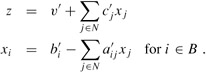
Suppose that SIMPLEX returns values ![]() on the primal linear program (A, b, c). Let N and B denote the nonbasic and basic variables for the final slack form, let c′ denote the coefficients in the final slack form, and let
on the primal linear program (A, b, c). Let N and B denote the nonbasic and basic variables for the final slack form, let c′ denote the coefficients in the final slack form, and let ![]() be defined by equation (29.94). Then
be defined by equation (29.94). Then ![]() is an optimal solution to the primal linear program,
is an optimal solution to the primal linear program, ![]() is an optimal solution to the dual linear program, and
is an optimal solution to the dual linear program, and
Proof By Corollary 29.9, if we can find feasible solutions ![]() and
and ![]() that satisfy equation (29.95), then
that satisfy equation (29.95), then ![]() and
and ![]() must be optimal primal and dual solutions. We shall now show that the solutions
must be optimal primal and dual solutions. We shall now show that the solutions ![]() and
and ![]() described in the statement of the theorem satisfy equation (29.95).
described in the statement of the theorem satisfy equation (29.95).
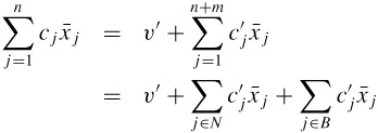
Suppose that we run SIMPLEX on a primal linear program, as given in lines (29.16)-(29.18). The algorithm proceeds through a series of slack forms until it terminates with a final slack form with objective function
Since SIMPLEX terminated with a solution, by the condition in line 2 we know that
If we define
we can rewrite equation (29.96) as
| (29.99) | 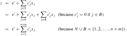 |
For the basic solution ![]() associated with this final slack form,
associated with this final slack form, ![]() for all j ∈ N, and z = v′. Since all slack forms are equivalent, if we evaluate the original objective function on
for all j ∈ N, and z = v′. Since all slack forms are equivalent, if we evaluate the original objective function on ![]() , we must obtain the same objective value, i.e.,
, we must obtain the same objective value, i.e.,
| (29.101) | 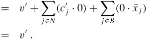 |
We shall now show that ![]() , defined by equation (29.94), is feasible for the dual linear program and that its objective value
, defined by equation (29.94), is feasible for the dual linear program and that its objective value ![]() equals
equals ![]() . Equation (29.100) says that the first and last slack forms, evaluated at
. Equation (29.100) says that the first and last slack forms, evaluated at ![]() , are equal. More generally, the equivalence of all slack forms implies that for any set of values x = (x1, x2, ..., xn), we have
, are equal. More generally, the equivalence of all slack forms implies that for any set of values x = (x1, x2, ..., xn), we have
Therefore, for any set of values x, we have
so that
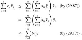
Applying Lemma 29.3 to equation (29.102), we obtain
By equation (29.103), we have that ![]() , and hence the objective value of the dual
, and hence the objective value of the dual ![]() is equal to that of the primal (v′). It remains to show that the solution
is equal to that of the primal (v′). It remains to show that the solution ![]() is feasible for the dual problem. From (29.97) and (29.98), we have that
is feasible for the dual problem. From (29.97) and (29.98), we have that ![]() for all j = 1, 2, ..., n + m. Hence, for any i = 1, 2, ..., m, (29.104) implies that
for all j = 1, 2, ..., n + m. Hence, for any i = 1, 2, ..., m, (29.104) implies that
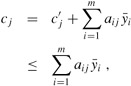
which satisfies the constraints (29.87) of the dual. Finally, since ![]() for each j ∈ N ∪ B, when we set
for each j ∈ N ∪ B, when we set ![]() according to equation (29.94), we have that each
according to equation (29.94), we have that each ![]() , and so the nonnegativity constraints are satisfied as well.
, and so the nonnegativity constraints are satisfied as well.
We have shown that, given a feasible linear program, if INITIALIZE-SIMPLEX returns a feasible solution, and if SIMPLEX terminates without returning "unbounded," then the solution returned is indeed an optimal solution. We have also shown how to construct an optimal solution to the dual linear program.
Suppose that we have a linear program that is not in standard form. We could produce the dual by first converting it to standard form, and then taking the dual. It would be more convenient, however, to be able to produce the dual directly. Explain how, given an arbitrary linear program, we can directly take the dual of that linear program.
Write down the dual of the maximum-flow linear program, as given in lines (29.47)-(29.50). Explain how to interpret this formulation as a minimum-cut problem.
Write down the dual of the minimum-cost-flow linear program, as given in lines (29.51)-(29.55). Explain how to interpret this problem in terms of graphs and flows.
|
|
< Day Day Up > |
|