An example of the simplex algorithm

We begin with an extended example. Consider the following linear program in standard form:

(29.56)

subject to

(29.57)

(29.58)

(29.59)

(29.60)

In order to use the simplex algorithm, we must convert the linear program into slack form; we saw how to do so in Section 29.1. In addition to being an algebraic manipulation, slack is a useful algorithmic concept. Recalling from Section 29.1 that each variable has a corresponding nonnegativity constraint, we say that an equality constraint is tight for a particular setting of its nonbasic variables if they cause the constraint's basic variable to become 0. Similarly, a setting of the nonbasic variables that would make a basic variable become negative violates that constraint. Thus, the slack variables explicitly maintain how far each constraint is from being tight, and so they help to determine how much we can increase values of nonbasic values without violating any constraints.

Associating the slack variables x₄, x₅, and x₆ with inequalities (29.57)-(29.59), respectively, and putting the linear program into slack form, we obtain

(29.61)

(29.62)

(29.63)

(29.64)

The system of constraints (29.62)-(29.64) has 3 equations and 6 variables. Any setting of the variables x₁, x₂, and x₃ defines values for x₄, x₅, and x₆; there are therefore an infinite number of solutions to this system of equations. A solution is feasible if all of x₁, x₂, ..., x₆ are nonnegative, and there can be an infinite number of feasible solutions as well. The infinite number of possible solutions to a system such as this one will be useful in later proofs. We will focus on the basic solution: set all the (nonbasic) variables on the right-hand side to 0 and then compute the values of the (basic) variables on the left-hand side. In this example, the basic solution is and it has objective value z = (3 · 0) + (1 · 0) + (2 · 0) = 0. Observe that this basic solution sets for each i ∈ B. An iteration of the simplex algorithm will rewrite the set of equations and the objective function so as to put a different set of variables on the right-hand side. Thus, there will be a different basic solution associated with the rewritten problem. We emphasize that the rewrite does not in any way change the underlying linear-programming problem; the problem at one iteration has the identical set of feasible solutions as the problem at the previous iteration. The problem does, however, have a different basic solution than that of the previous iteration.

If a basic solution is also feasible, we call it a basic feasible solution. During the running of the simplex algorithm, the basic solution will almost always be a basic feasible solution. We shall see in Section 29.5, however, that for the first few iterations of the simplex algorithm, the basic solution may not be feasible.

Our goal, in each iteration, is to reformulate the linear program so that the basic solution has a greater objective value. We select a nonbasic variable x_e whose coefficient in the objective function is positive, and we increase the value of x_e as much as possible without violating any of the constraints. The variable x_e becomes basic, and some other variable x_l becomes nonbasic. The values of other basic variables and of the objective function may also change.

To continue the example, let's think about increasing the value of x₁. As we increase x₁, the values of x₄, x₅, and x₆ all decrease. Because we have a nonnegativity constraint for each variable, we cannot allow any of them to become negative. If x₁ increases above 30, then x₄ becomes negative, while x₅ and x₆ become negative when x₁ increases above 12 and 9 respectively. The third constraint (29.64) is the tightest constraint, and it limits how much we can increase x₁. We will, therefore, switch the roles of x₁ and x₆. We solve equation (29.64) for x₁ and obtain

(29.65)

To rewrite the other equations with x₆ on the right-hand side, we substitute for x₁ using equation (29.65). Doing so for equation (29.62), we obtain

(29.66)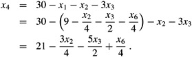

Similarly, we can combine equation (29.65) with constraint (29.63) and with objective function (29.61) to rewrite our linear program in the following form:

(29.67)

(29.68)

(29.69)

(29.70)

We call this operation a pivot. As demonstrated above, a pivot chooses a nonbasic variable x_e, called the entering variable, and a basic variable x_l, called the leaving variable, and exchanges their roles.

The linear program described in (29.67)-(29.70) is equivalent to the linear program described in equations (29.61)-(29.64). The operations we perform in the simplex algorithm are rewriting equations so that variables move between the left-hand side and the right-hand side, and substituting one equation into another. The first operation trivially creates an equivalent problem, and the second, by elementary linear algebra, also creates an equivalent problem.

To demonstrate this equivalence, observe that our original basic solution (0, 0, 0, 30, 24, 36) satisfies the new equations (29.68)-(29.70) and has objective value 27 + (1/4) · 0 + (1/2) · 0 - (3/4) · 36 = 0. The basic solution associated with the new linear program sets the nonbasic values to 0 and is (9, 0, 0, 21, 6, 0), with objective value z = 27. Simple arithmetic verifies that this solution also satisfies equations (29.62)-(29.64) and, when plugged into objective function (29.61), has objective value (3 · 9) + (1 · 0) + (2 · 0) = 27.

Continuing the example, we wish to find a new variable whose value we wish to increase. We do not want to increase x₆, since as its value increases, the objective value decreases. We can attempt to increase either x₂ or x₃; we will choose x₃. How far can we increase x₃ without violating any of the constraints? Constraint (29.68) limits it to 18, constraint (29.69) limits it to 42/5, and constraint (29.70) limits it to 3/2. The third constraint is again the tightest one, and we will therefore rewrite the third constraint so that x₃ is on the left-hand side and x₅ is on the right-hand side. We then substitute this new equation into equations (29.67)-(29.69) and obtain the new, but equivalent, system

(29.71)

(29.72)

(29.73)

(29.74)

This system has the associated basic solution (33/4, 0, 3/2, 69/4, 0, 0), with objective value 111/4. Now the only way to increase the objective value is to increase x₂. The three constraints give upper bounds of 132, 4, and ∞, respectively. (The upper bound of ∞ from constraint (29.74) is because as we increase x₂, the value of the basic variable x₄ increases also. This constraint, therefore, places no restriction on how much x₂ can be increased.) We increase x₂ to 4, and it becomes nonbasic. Then we solve equation (29.73) for x₂ and substitute in the other equations to obtain

(29.75)

(29.76)

(29.77)

(29.78)

At this point, all coefficients in the objective function are negative. As we shall see later in this chapter, this situation occurs only when we have rewritten the linear program so that the basic solution is an optimal solution. Thus, for this problem, the solution (8, 4, 0, 18, 0, 0), with objective value 28, is optimal. We can now return to our original linear program given in (29.56)-(29.60). The only variables in the original linear program are x₁, x₂, and x₃, and so our solution is x₁ = 8, x₂ = 4, and x₃ = 0, with objective value (3 · 8) + (1 · 4) + (2 · 0) = 28. Note that the values of the slack variables in the final solution measure how much slack is in each inequality. Slack variable x₄ is 18, and in inequality (29.57), the left-hand side, with value 8 + 4 + 0 = 12, is 18 less than the right-hand side of 30. Slack variables x₅ and x₆ are 0 and indeed, in inequalities (29.58) and (29.59), the left-hand and right-hand sides are equal. Observe also that even though the coefficients in the original slack form are integral, the coefficients in the other linear programs are not necessarily integral, and the intermediate solutions are not necessarily integral. Furthermore, the final solution to a linear program need not be integral; it is purely coincidental that this example has an integral solution.

Pivoting

We now formalize the procedure for pivoting. The procedure PIVOT takes as input a slack form, given by the tuple (N, B, A, b, c, v), the index l of the leaving variable x_l, and the index e of the entering variable x_e. It returns the tuple describing the new slack form. (Recall again that the entries of the matrices A and are actually the negative of the coefficients that appear in the slack form.)

PIVOT(N, B, A, b, c, v, l, e)
 1 ▹ Compute the coefficients of the equation for new basic variable xe.
 2 
 3 for each j ∈ N - {e}
 4     do 
 5 
 6 ▹ Compute the coefficients of the remaining constraints.
 7 for each i ∈ B - {l}
 8     do 
 9        for each j ∈ N - {e}
10           do 
11        
12 ▹ Compute the objective function.
13 
14 for each j ∈ N - {e}
15     do 
16 
17 ▹ Compute new sets of basic and nonbasic variables.
18 
19 
20 return 

PIVOT works as follows. Lines 2-5 compute the coefficients in the new equation for x_e by rewriting the equation that has x_l on the left-hand side to instead have x_e on the left-hand side. Lines 7-11 update the remaining equations by substituting the right-hand side of this new equation for each occurrence of x_e. Lines 13-16 do the same substitution for the objective function, and lines 18 and 19 update the sets of nonbasic and basic variables. Line 20 returns the new slack form. As given, if a_le = 0, PIVOT would cause an error by dividing by 0, but as we shall see in the proofs of Lemmas 29.2 and 29.12, PIVOT is called only when a_le ≠ 0.

We now summarize the effect that PIVOT has on the values of the variables in the basic solution.

Lemma 29.1

Consider a call to PIVOT(N, B, A, b, c, v, l, e) in which a_le ≠ 0. Let the values returned from the call be , and let denote the basic solution after the call. Then

1. for each .

2. .

3. for each .

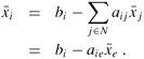
Proof The first statement is true because the basic solution always sets all nonbasic variables to 0. When we set each nonbasic variable to 0 in a constraint

we have that for each . Since , by line 2 of PIVOT, we have

which proves the second statement. Similarly, using line 8 for each , we have

which proves the third statement.

The formal simplex algorithm

We are now ready to formalize the simplex algorithm, which we demonstrated by example. That example was a particularly nice one, and we could have had several other issues to address:

• How do we determine if a linear program is feasible?

• What do we do if the linear program is feasible, but the initial basic solution is not feasible?

• How do we determine if a linear program is unbounded?

• How do we choose the entering and leaving variables?

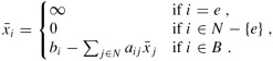
In Section 29.5, we shall show how to determine if a problem is feasible, and if so, how to find a slack form in which the initial basic solution is feasible. We therefore assume that we have a procedure INITIALIZE-SIMPLEX(A, b, c) that takes as input a linear program in standard form, that is, an m × n matrix A = (a_ij), an m-dimensional vector b = (b_i), and an n-dimensional vector c = (c_j). If the problem is infeasible, it returns a message that the program is infeasible and then terminates. Otherwise, it returns a slack form for which the initial basic solution is feasible.

The procedure SIMPLEX takes as input a linear program in standard form, as just described. It returns an n-vector that is an optimal solution to the linear program described in (29.19)-(29.21).

SIMPLEX(A, b, c)
 1  (N, B, A, b, c, v) ← INITIALIZE-SIMPLEX(A, b, c)
 2  while some index j ∈ N has cj > 0
 3      do choose an index e ∈ N for which ce > 0
 4         for each index i ∈ B
 5             do if aie > 0
 6                   then Δi ← bi/aie
 7                   else Δi ← ∞
 8         choose an index l ∈ B that minimizes Δi
 9         if Δl = ∞
10            then return "unbounded"
11            else (N, B, A, b, c, v) ← PIVOT(N, B, A, b, c, v, l, e)
12  for i ← 1 to n
13       do if i ∈ B
14             then 
15             else 
16  return 

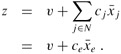
The SIMPLEX procedure works as follows. In line 1, it calls the procedure INITIALIZE-SIMPLEX(A, b, c), described above, which either determines that the linear program is infeasible or returns a slack form for which the basic solution is feasible. The main part of the algorithm is given in the while loop in lines 2-11. If all the coefficients in the objective function are negative, then the while loop terminates. Otherwise, in line 3, we select a variable x_e whose coefficient in the objective function is positive to be the entering variable. While we have the freedom to choose any such variable as the entering variable, we assume that we use some prespecified deterministic rule. Next, in lines 4-8, we check each constraint, and we pick the one that most severely limits the amount by which we can increase x_e without violating any of the nonnegativity constraints; the basic variable associated with this constraint is x_l. Again, we may have the freedom to choose one of several variables as the leaving variable, but we assume that we use some prespecified deterministic rule. If none of the constraints limits the amount by which the entering variable can increase, the algorithm returns "unbounded" in line 10. Otherwise, line 11 exchanges the roles of the entering and leaving variables by calling the subroutine PIVOT(N, B, A, b, c, v, l, e), described above. Lines 12-15 compute a solution for the original linear-programming variables by setting all the nonbasic variables to 0 and each basic variable to b_i. In Theorem 29.10, we shall see that this solution is an optimal solution to the linear program. Finally, line 16 returns the computed values of these original linear-programming variables.

To show that SIMPLEX is correct, we first show that if SIMPLEX has an initial feasible solution and eventually terminates, then it either returns a feasible solution or determines that the linear program is unbounded. Then, we show that SIMPLEX terminates. Finally, in Section 29.4, we show that the solution returned is optimal.

Lemma 29.2

Given a linear program (A, b, c), suppose that the call to INITIALIZE-SIMPLEX in line 1 of SIMPLEX returns a slack form for which the basic solution is feasible. Then if SIMPLEX returns a solution in line 16, that solution is a feasible solution to the linear program. If SIMPLEX returns "unbounded" in line 10, the linear program is unbounded.

Proof We use the following three-part loop invariant:

• At the start of each iteration of the while loop of lines 2-11,

  1. the slack form is equivalent to the slack form returned by the call of INITIALIZE-SIMPLEX,

  2. for each i ∈ B, we have b_i ≥ 0, and

  3. the basic solution associated with the slack form is feasible.

• Initialization: The equivalence of the slack forms is trivial for the first iteration. We assume, in the statement of the lemma, that the call to INITIALIZE-SIMPLEX in line 1 of SIMPLEX returns a slack form for which the basic solution is feasible. Thus, the third part of the invariant is true. Furthermore, since each basic variable x_i is set to b_i in the basic solution, and the feasibility of the basic solution implies that each basic variable x_i is nonnegative, we have that b_i ≥ 0. Thus, the second part of the invariant holds.

• Maintenance: We shall show that the loop invariant is maintained, assuming that the return statement in line 10 is not executed. We shall handle the case that line 10 executes when we discuss termination.

  An iteration of the while loop exchanges the role of a basic and a nonbasic variable. The only operations performed involve solving equations and substituting one equation into another, and therefore the slack form is equivalent to the one from the previous iteration which, by the loop invariant, is equivalent to the initial slack form.

  We now demonstrate the second part of the loop invariant. We assume that at the start of each iteration of the while loop, b_i ≥ 0 for each i ∈ B, and we shall show that that these inequalities remain true after the call to PIVOT in line 11. Since the only changes to the variables b_i and the set B of basic variables occur in this assignment, it suffices to show that line 11 maintains this part of the invariant. We let b_i, a_ij, and B refer to values before the call of PIVOT, and refer to values returned from PIVOT.

  First, we observe that because b_l ≥ 0 by the loop invariant, a_le > 0 by line 5 of SIMPLEX, and by line 2 of PIVOT.

  For the remaining indices i ∈ B - l, we have that

  (29.79)

  We have two cases to consider, depending on whether a_ie > 0 or a_ie ≤ 0. If a_ie > 0, then since we chose l such that

  (29.80)

  we have

  	=	bi - aie(bl/ale)	(by equation (29.79))
  	≥	bi - aie(bi/aie)	(by inequality (29.80))
  	=	bi - bi
  	=	0,

  and thus . If a_ie = 0, then because a_le, b_i, and b_l are all nonnegative, equation (29.79) implies that must be nonnegative, too.

  We now argue that the basic solution is feasible, i.e., that all variables have nonnegative values. The nonbasic variables are set to 0 and thus are nonnegative. Each basic variable x_i is defined by the equation

  

  The basic solution sets . Using the second part of the loop invariant, we conclude that each basic variable is nonnegative.

• Termination: The while loop can terminate in one of two ways. If it terminates because of the condition in line 2, then the current basic solution is feasible and this solution is returned in line 16. The other way to terminate is to return "unbounded" in line 10. In this case, for each iteration of the for loop in lines 4-7, when line 5 is executed, we find that a_ie ≤ 0. Let x be the basic solution associated with the slack form at the beginning of the iteration that returned "unbounded." Consider the solution defined as

  

  We now show that this solution is feasible, i.e., that all variables are nonnegative. The nonbasic variables other than are 0, and is positive; thus all nonbasic variables are nonnegative. For each basic variable , we have

  

  The loop invariant implies that b_i ≥ 0, and we have a_ie ≤ 0 and . Thus, .

  Now we show that the objective value for the solution is unbounded. The objective value is

  

  Since c_e > 0 (by line 3) and , the objective value is ∞, and thus the linear program is unbounded.

At each iteration, SIMPLEX maintains A, b, c, and v in addition to the sets N and B. Although explicitly maintaining A, b, c, and v is essential for the efficient implementation of the simplex algorithm, it is not strictly necessary. In other words, the slack form is uniquely determined by the sets of basic and nonbasic variables. Before proving this fact, we prove a useful algebraic lemma.

Lemma 29.3

Let I be a set of indices. For each i ∈ I, let α_i and β_i be real numbers, and let x_i be a real-valued variable. Let γ be any real number. Suppose that for any settings of the x_i, we have

(29.81)

Then α_i = β_i for each i ∈ I, and γ = 0.

Proof Since equation (29.81) holds for any values of the x_i, we can use particular values to draw conclusions about α, β, and γ. If we let x_i = 0 for each i ∈ I, we conclude that γ = 0. Now pick an arbitrary index i ∈ I, and set x_i = 1 and x_k = 0 for all k ≠ i. Then we must have α_i = β_i. Since we picked i as any index in i, we conclude that α_i = β_i for each i ∈ I.

We now show that the slack form of a linear program is uniquely determined by the set of basic variables.

Lemma 29.4

Let (A, b, c) be a linear program in standard form. Given a set B of basic variables, the associated slack form is uniquely determined.

Proof Assume for purpose of contradiction that there are two different slack forms with the same set B of basic variables. The slack forms must also have identical sets N = {1, 2, ..., n + m} - B of nonbasic variables. We write the first slack form as

(29.82)

(29.83)

and the second as

(29.84)

(29.85)

Consider the system of equations formed by subtracting each equation in line (29.85) from the corresponding equation in line (29.83). The resulting system is

or, equivalently,

Now, for each i ∈ B, apply Lemma 29.3 with α_i = a_ij, , and . Since α_i = β_i, we have that for each j ∈ N, and since γ = 0, we have that . Thus, for the two slack forms, A and b are identical to A′ and b′. Using a similar argument, Exercise 29.3-1 shows that it must also be the case that c = c′ and v = v′, and hence that the slack forms must be identical.

It remains to show that SIMPLEX terminates, and when it does terminate, the solution returned is optimal. Section 29.4 will address optimality. We now discuss termination.

Termination

In the example given in the beginning of this section, each iteration of the simplex algorithm increased the objective value associated with the basic solution. As Exercise 29.3-2 asks you to show, no iteration of SIMPLEX can decrease the objective value associated with the basic solution. Unfortunately, it is possible that an iteration leaves the objective value unchanged. This phenomenon is called degeneracy and we now study it in greater detail.

The objective value is changed by the assignment in line 13 of PIVOT. Since SIMPLEX calls PIVOT only when c_e > 0, the only way for the objective value to remain unchanged (i.e., ) is for to be 0. This value is assigned as in line 2 of PIVOT. Since we always call PIVOT with a_le ≠ 0, we see that for to equal 0, and hence the objective value to be unchanged, we must have b_l = 0.

Indeed, this situation can occur. Consider the linear program

Suppose that we choose x₁ as the entering variable and x₄ as the leaving variable. After pivoting, we obtain

At this point, our only choice is to pivot with x₃ entering and x₅ leaving. Since b₅ = 0, the objective value of 8 remains unchanged after pivoting:

The objective value has not changed, but our representation has. Fortunately, if we pivot again, with x₂ entering and x₁ leaving, the objective value will increase, and the simplex algorithm can continue.

We now show that degeneracy is the only thing that could possibly keep the simplex algorithm from terminating. Recall our assumption that SIMPLEX chooses indices e and l, in lines 3 and 8 respectively, according to some deterministic rule. We say that SIMPLEX cycles if the slack forms at two different iterations are identical, in which case, since SIMPLEX is a deterministic algorithm, it will cycle through the same series of slack forms forever.

Lemma 29.5

If SIMPLEX fails to terminate in at most iterations, then it cycles.

Proof By Lemma 29.4, the set B of basic variables uniquely determines a slack form. There are n + m variables and |B| = m, and therefore there are ways to choose B. Thus, there are only unique slack forms. Therefore, if SIMPLEX runs for more than iterations, it must cycle.

Cycling is theoretically possible, but extremely rare. It is avoidable by choosing the entering and leaving variables somewhat more carefully. One option is to perturb the input slightly so that it is impossible to have two solutions with the same objective value. A second is to break ties lexicographically, and a third is to break ties by always choosing the variable with the smallest index. This last strategy is known as Bland's rule. We omit the proof that these strategies avoid cycling.

Lemma 29.6

If in lines 3 and 8 of SIMPLEX, ties are always broken by choosing the variable with the smallest index, then SIMPLEX must terminate.

We conclude this section with the following lemma.

Lemma 29.7

Assuming that INITIALIZE-SIMPLEX returns a slack form for which the basic solution is feasible, SIMPLEX either reports that a linear program is unbounded, or it terminates with a feasible solution in at most iterations.

Proof Lemmas 29.2 and 29.6 show that if INITIALIZE-SIMPLEX returns a slack form for which the basic solution is feasible, SIMPLEX either reports that a linear program is unbounded, or it terminates with a feasible solution. By the contra-positive of Lemma 29.5, if SIMPLEX terminates with a feasible solution, then it terminates in at most iterations.

Exercises 29.3-1

Complete the proof of Lemma 29.4 by showing that it must be the case that c = c′ and v = v′.

Exercises 29.3-2

Show that the call to PIVOT in line 11 of SIMPLEX will never decrease the value of v.

Exercises 29.3-3

Suppose we convert a linear program (A, b, c) in standard form to slack form. Show that the basic solution is feasible if and only if b_i ≥ 0 for i = 1, 2, ..., m.

Exercises 29.3-4

Solve the following linear program using SIMPLEX:

maximize	18x1	+	12.5x2
subject to
	x1	+	x2	≤	20
	x1			≤	12
			x2	≤	16
	x1, x2			≥	0.

Exercises 29.3-5

Solve the following linear program using SIMPLEX:

maximize	-5x1	-	3x2
subject to
	x1	-	x2	≤	1
	2x1	+	x2	≤	2
	x1, x2			≥	0.

Exercises 29.3-6

Solve the following linear program using SIMPLEX:

minimize	x1	+	x2	+	x3
subject to
	2x1	+	7.5x2	+	3x3	≥	10000
	20x1	+	5x2	+	10x3	≥	30000
	x1, x2, x3					≥	0.