35.1 The vertex-cover problem

The vertex-cover problem was defined and proven NP-complete in Section 34.5.2. A vertex cover of an undirected graph G = (V, E) is a subset V′ ⊆ V such that if (u, v) is an edge of G, then either u ∈ V′ or v ∈ V′ (or both). The size of a vertex cover is the number of vertices in it.

The vertex-cover problem is to find a vertex cover of minimum size in a given undirected graph. We call such a vertex cover an optimal vertex cover. This problem is the optimization version of an NP-complete decision problem.

Even though it may be difficult to find an optimal vertex cover in a graph G, it is not too hard to find a vertex cover that is near-optimal. The following approximation algorithm takes as input an undirected graph G and returns a vertex cover whose size is guaranteed to be no more than twice the size of an optimal vertex cover.

APPROX-VERTEX-COVER(G">
1  C ← Ø
2  E′ ← E[G]
3  while E′ ≠ Ø
4     do let (u, v) be an arbitrary edge of E′
5        C ← C ∪ {u, v}
6        remove from E′ every edge incident on either u or v
7  return C

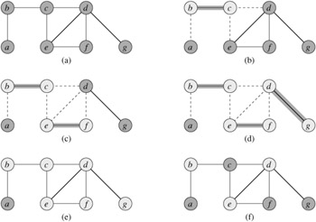
Figure 35.1 illustrates the operation of APPROX-VERTEX-COVER. The variable C contains the vertex cover being constructed. Line 1 initializes C to the empty set. Line 2 sets E′ to be a copy of the edge set E[G] of the graph. The loop on lines 3-6 repeatedly picks an edge (u, v) from E′, adds its endpoints u and v to C, and deletes all edges in E′ that are covered by either u or v. The running time of this algorithm is O(V + E), using adjacency lists to represent E′.

Figure 35.1: The operation of APPROX-VERTEX-COVER. (a) The input graph G, which has 7 vertices and 8 edges. (b) The edge (b, c), shown heavy, is the first edge chosen by APPROX-VERTEX-COVER. Vertices b and c, shown lightly shaded, are added to the set C containing the vertex cover being created. Edges (a, b), (c, e), and (c, d), shown dashed, are removed since they are now covered by some vertex in C. (c) Edge (e, f) is chosen; vertices e and f are added to C. (d) Edge (d, g) is chosen; vertices d and g are added to C. (e) The set C, which is the vertex cover produced by APPROX-VERTEX-COVER, contains the six vertices b, c, d, e, f, g. (f) The optimal vertex cover for this problem contains only three vertices: b, d, and e.

Theorem 35.1

APPROX-VERTEX-COVER is a polynomial-time 2-approximation algorithm.

Proof We have already shown that APPROX-VERTEX-COVER runs in polynomial time.

The set C of vertices that is returned by APPROX-VERTEX-COVER is a vertex cover, since the algorithm loops until every edge in E[G] has been covered by some vertex in C.

To see that APPROX-VERTEX-COVER returns a vertex cover that is at most twice the size of an optimal cover, let A denote the set of edges that were picked in line 4 of APPROX-VERTEX-COVER. In order to cover the edges in A, any vertex cover-in particular, an optimal cover C*-must include at least one endpoint of each edge in A. No two edges in A share an endpoint, since once an edge is picked in line 4, all other edges that are incident on its endpoints are deleted from E′ in line 6. Thus, no two edges in A are covered by the same vertex from C*, and we have the lower bound

(35.2)

on the size of an optimal vertex cover. Each execution of line 4 picks an edge for which neither of its endpoints is already in C, yielding an upper bound (an exact upper bound, in fact) on the size of the vertex cover returned:

(35.3)

Combining equations (35.2) and (35.3), we obtain

\|C\|	=	2\|A\|
	≤	2\|C*\|,

thereby proving the theorem.

Let us reflect on this proof. At first one might wonder how it is possible to prove that the size of the vertex cover returned by APPROX-VERTEX-COVER is at most twice the size of an optimal vertex cover, since we do not know what the size of the optimal vertex cover is. The answer is that we utilize a lower bound on the optimal vertex cover. As Exercise 35.1-2 asks you to show, the set A of edges that were picked in line 4 of APPROX-VERTEX-COVER is actually a maximal matching in the graph G. (A maximal matching is a matching that is not a proper subset of any other matching.) The size of a maximal matching is, as we argued in the proof of Theorem 35.1, a lower bound on the size of an optimal vertex cover. The algorithm returns a vertex cover whose size is at most twice the size of the maximal matching A. By relating the size of the solution returned to the lower bound, we obtain our approximation ratio. We will use this methodology in later sections as well.

Exercises 35.1-1

Give an example of a graph for which APPROX-VERTEX-COVER always yields a suboptimal solution.

Exercises 35.1-2

Let A denote the set of edges that were picked in line 4 of APPROX-VERTEX-COVER. Prove that the set A is a maximal matching in the graph G.

Exercises 35.1-3: ⋆

Professor Nixon proposes the following heuristic to solve the vertex-cover problem. Repeatedly select a vertex of highest degree, and remove all of its incident edges. Give an example to show that the professor's heuristic does not have an approximation ratio of 2. (Hint: Try a bipartite graph with vertices of uniform degree on the left and vertices of varying degree on the right.)

Exercises 35.1-4

Give an efficient greedy algorithm that finds an optimal vertex cover for a tree in linear time.

Exercises 35.1-5

From the proof of Theorem 34.12, we know that the vertex-cover problem and the NP-complete clique problem are complementary in the sense that an optimal vertex cover is the complement of a maximum-size clique in the complement graph. Does this relationship imply that there is a polynomial-time approximation algorithm with a constant approximation ratio for the clique problem? Justify your answer.

\|C\|	=	2\|A\|
	≤	2\|C*\|,