|
|
< Day Day Up > |
|
In the traveling-salesman problem introduced in Section 34.5.4, we are given a complete undirected graph G = (V, E) that has a nonnegative integer cost c(u, v) associated with each edge (u, v) ∈ E, and we must find a hamiltonian cycle (a tour) of G with minimum cost. As an extension of our notation, let c(A) denote the total cost of the edges in the subset A ⊆ E:
In many practical situations, it is always cheapest to go directly from a place u to a place w; going by way of any intermediate stop v can't be less expensive. Putting it another way, cutting out an intermediate stop never increases the cost. We formalize this notion by saying that the cost function c satisfies the triangle inequality if for all vertices u, v, w ∈ V,
c(u, w) ≤ c(u, v) + c(v, w).
The triangle inequality is a natural one, and in many applications it is automatically satisfied. For example, if the vertices of the graph are points in the plane and the cost of traveling between two vertices is the ordinary euclidean distance between them, then the triangle inequality is satisfied. (There are many cost functions other than euclidean distance that satisfy the triangle inequality.)
As Exercise 35.2-2 shows, the traveling-salesman problem is NP-complete even if we require that the cost function satisfy the triangle inequality. Thus, it is unlikely that we can find a polynomial-time algorithm for solving this problem exactly. We therefore look instead for good approximation algorithms.
In Section 35.2.1, we examine a 2-approximation algorithm for the traveling-salesman problem with the triangle inequality. In Section 35.2.2, we show that without the triangle inequality, a polynomial-time approximation algorithm with a constant approximation ratio does not exist unless P = NP.
Applying the methodology of the previous section, we will first compute a structure-a minimum spanning tree-whose weight is a lower bound on the length of an optimal traveling-salesman tour. We will then use the minimum spanning tree to create a tour whose cost is no more than twice that of the minimum spanning tree's weight, as long as the cost function satisfies the triangle inequality. The following algorithm implements this approach, calling the minimum-spanning-tree algorithm MST-PRIM from Section 23.2 as a subroutine.
APPROX-TSP-TOUR(G, c">
1  select a vertex r ∈ V [G] to be a "root" vertex
2  compute a minimum spanning tree T for G from root r
       using MST-PRIM(G, c, r)
3  let L be the list of vertices visited in a preorder tree walk of T
4  return the hamiltonian cycle H that visits the vertices in the order L
Recall from Section 12.1 that a preorder tree walk recursively visits every vertex in the tree, listing a vertex when it is first encountered, before any of its children are visited.
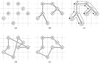
Figure 35.2 illustrates the operation of APPROX-TSP-TOUR. Part (a) of the figure shows the given set of vertices, and part (b) shows the minimum spanning tree T grown from root vertex a by MST-PRIM. Part (c) shows how the vertices are visited by a preorder walk of T , and part (d) displays the corresponding tour, which is the tour returned by APPROX-TSP-TOUR. Part (e) displays an optimal tour, which is about 23% shorter.
By Exercise 23.2-2, even with a simple implementation of MST-PRIM, the running time of APPROX-TSP-TOUR is 0398(V2). We now show that if the cost function for an instance of the traveling-salesman problem satisfies the triangle inequality, then APPROX-TSP-TOUR returns a tour whose cost is not more than twice the cost of an optimal tour.
APPROX-TSP-TOUR is a polynomial-time 2-approximation algorithm for the traveling-salesman problem with the triangle inequality.
Proof We have already shown that APPROX-TSP-TOUR runs in polynomial time.
Let H* denote an optimal tour for the given set of vertices. Since we obtain a spanning tree by deleting any edge from a tour, the weight of the minimum spanning tree T is a lower bound on the cost of an optimal tour, that is,
A full walk of T lists the vertices when they are first visited and also whenever they are returned to after a visit to a subtree. Let us call this walk W . The full walk of our example gives the order
a, b, c, b, h, b, a, d, e, f, e, g, e, d, a.
Since the full walk traverses every edge of T exactly twice, we have (extending our definition of the cost c in the natural manner to handle multisets of edges)
Equations (35.4) and (35.5) imply that
and so the cost of W is within a factor of 2 of the cost of an optimal tour.
Unfortunately, W is generally not a tour, since it visits some vertices more than once. By the triangle inequality, however, we can delete a visit to any vertex from W and the cost does not increase. (If a vertex v is deleted from W between visits to u and w, the resulting ordering specifies going directly from u to w.) By repeatedly applying this operation, we can remove from W all but the first visit to each vertex. In our example, this leaves the ordering
This ordering is the same as that obtained by a preorder walk of the tree T. Let H be the cycle corresponding to this preorder walk. It is a hamiltonian cycle, since every vertex is visited exactly once, and in fact it is the cycle computed by APPROX-TSP-TOUR. Since H is obtained by deleting vertices from the full walk W , we have
Combining inequalities (35.6) and (35.7) shows that c(H) ≤ 2c(H*), which completes the proof.
In spite of the nice approximation ratio provided by Theorem 35.2, APPROX-TSP-TOUR is usually not the best practical choice for this problem. There are other approximation algorithms that typically perform much better in practice. See the references at the end of this chapter.
If we drop the assumption that the cost function c satisfies the triangle inequality, good approximate tours cannot be found in polynomial time unless P = NP.
If P ≠ NP, then for any constant ρ ≥ 1, there is no polynomial-time approximation algorithm with approximation ratio ρ for the general traveling-salesman problem.
Proof The proof is by contradiction. Suppose to the contrary that for some number ρ ≥ 1, there is a polynomial-time approximation algorithm A with approximation ratio ρ. Without loss of generality, we assume that ρ is an integer, by rounding it up if necessary. We shall then show how to use A to solve instances of the hamiltonian-cycle problem (defined in Section 34.2) in polynomial time. Since the hamiltonian-cycle problem is NP-complete, by Theorem 34.13, solving it in polynomial time implies that P = NP, by Theorem 34.4.
Let G = (V, E) be an instance of the hamiltonian-cycle problem. We wish to determine efficiently whether G contains a hamiltonian cycle by making use of the hypothesized approximation algorithm A. We turn G into an instance of the traveling-salesman problem as follows. Let G′ = (V, E′) be the complete graph on V ; that is,
E′ = {(u, v) : u, v ∈ V and u ≠ v}.
Assign an integer cost to each edge in E′ as follows:
Representations of G′ and c can be created from a representation of G in time polynomial in |V | and |E|.
Now, consider the traveling-salesman problem (G′, c). If the original graph G has a hamiltonian cycle H , then the cost function c assigns to each edge of H a cost of 1, and so (G′, c) contains a tour of cost |V|. On the other hand, if G does not contain a hamiltonian cycle, then any tour of G′ must use some edge not in E. But any tour that uses an edge not in E has a cost of at least
|
(ρ | V | + 1) + (|V | - 1) |
= |
ρ|V | + |V | |
|
> |
ρ|V |. |
Because edges not in G are so costly, there is a gap of at least |V | between the cost of a tour that is a hamiltonian cycle in G (cost |V |) and the cost of any other tour (cost at least ρ|V | + |V |).
What happens if we apply the approximation algorithm A to the traveling-salesman problem (G′, c)? Because A is guaranteed to return a tour of cost no more than times the cost of an optimal tour, if G contains a hamiltonian cycle, then A must return it. If G has no hamiltonian cycle, then A returns a tour of cost more than ρ|V |. Therefore, we can use A to solve the hamiltonian-cycle problem in polynomial time.
The proof of Theorem 35.3 is an example of a general technique for proving that a problem cannot be approximated well. Suppose that given an NP-hard problem X, we can produce a minimization problem Y such that "yes" instances of X correspond to instances of Y with value at most k (for some k), but that "no" instances of X correspond to instances of Y with value greater than ρk. Then we have shown that, unless P = NP, there is no ρ-approximation algorithm for problem Y.
Suppose that a complete undirected graph G = (V, E) with at least 3 vertices has a cost function c that satisfies the triangle inequality. Prove that c(u, v) ≥ 0 for all u, v ∈ V.
Show how in polynomial time we can transform one instance of the traveling-salesman problem into another instance whose cost function satisfies the triangle inequality. The two instances must have the same set of optimal tours. Explain why such a polynomial-time transformation does not contradict Theorem 35.3, assuming that P ≠ NP.
Consider the following closest-point heuristic for building an approximate traveling-salesman tour. Begin with a trivial cycle consisting of a single arbitrarily chosen vertex. At each step, identify the vertex u that is not on the cycle but whose distance to any vertex on the cycle is minimum. Suppose that the vertex on the cycle that is nearest u is vertex v. Extend the cycle to include u by inserting u just after v. Repeat until all vertices are on the cycle. Prove that this heuristic returns a tour whose total cost is not more than twice the cost of an optimal tour.
The bottleneck traveling-salesman problem is the problem of finding the hamiltonian cycle such that the cost of the most costly edge in the cycle is minimized. Assuming that the cost function satisfies the triangle inequality, show that there exists a polynomial-time approximation algorithm with approximation ratio 3 for this problem. (Hint: Show recursively that we can visit all the nodes in a bottleneck spanning tree, as discussed in Problem 23-3, exactly once by taking a full walk of the tree and skipping nodes, but without skipping more than two consecutive intermediate nodes. Show that the costliest edge in a bottleneck spanning tree has a cost that is at most the cost of the costliest edge in a bottleneck hamiltonian cycle.)
|
|
< Day Day Up > |
|