|
|
< Day Day Up > |
|
A coin flip is an instance of a Bernoulli trial, which is defined as an experiment with only two possible outcomes: success, which occurs with probability p, and failure, which occurs with probability q = 1 - p. When we speak of Bernoulli trials collectively, we mean that the trials are mutually independent and, unless we specifically say otherwise, that each has the same probability p for success. Two important distributions arise from Bernoulli trials: the geometric distribution and the binomial distribution.
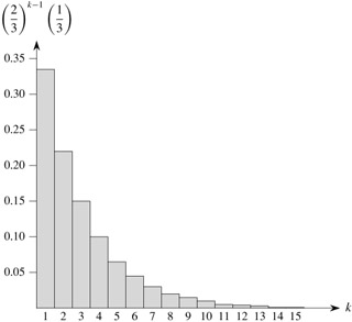
Suppose we have a sequence of Bernoulli trials, each with a probability p of success and a probability q = 1 - p of failure. How many trials occur before we obtain a success? Let the random variable X be the number of trials needed to obtain a success. Then X has values in the range {1, 2,...}, and for k ≥ 1,
since we have k - 1 failures before the one success. A probability distribution satisfying equation (C.30) is said to be a geometric distribution. Figure C.1 illustrates such a distribution.
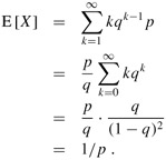
Assuming that q < 1, the expectation of a geometric distribution can be calculated using identity (A.8):
Thus, on average, it takes 1/ p trials before we obtain a success, an intuitive result. The variance, which can be calculated similarly, but using Exercise A.1-3, is
| (C.32) |
As an example, suppose we repeatedly roll two dice until we obtain either a seven or an eleven. Of the 36 possible outcomes, 6 yield a seven and 2 yield an eleven. Thus, the probability of success is p = 8/36 = 2/9, and we must roll 1/ p = 9/2 = 4.5 times on average to obtain a seven or eleven.
How many successes occur during n Bernoulli trials, where a success occurs with probability p and a failure with probability q = 1 - p? Define the random variable X to be the number of successes in n trials. Then X has values in the range {0,1,..., n}, and for k = 0,..., n,
since there are ![]() ways to pick which k of the n trials are successes, and the probability that each occurs is pkqn-k. A probability distribution satisfying equation (C.33) is said to be a binomial distribution. For convenience, we define the family of binomial distributions using the notation
ways to pick which k of the n trials are successes, and the probability that each occurs is pkqn-k. A probability distribution satisfying equation (C.33) is said to be a binomial distribution. For convenience, we define the family of binomial distributions using the notation
| (C.34) |
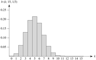
Figure C.2 illustrates a binomial distribution. The name "binomial" comes from the fact that (C.33) is the kth term of the expansion of (p + q)n. Consequently, since p + q = 1,
as is required by axiom 2 of the probability axioms.
We can compute the expectation of a random variable having a binomial distribution from equations (C.8) and (C.35). Let X be a random variable that follows the binomial distribution b(k; n, p), and let q = 1 - p. By the definition of expectation, we have
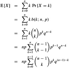
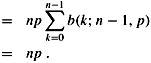
By using the linearity of expectation, we can obtain the same result with substantially less algebra. Let Xi be the random variable describing the number of successes in the ith trial. Then E[Xi] = p · 1 + q · 0 = p, and by linearity of expectation (equation (C.20)), the expected number of successes for n trials is
The same approach can be used to calculate the variance of the distribution. Using equation (C.26), we have ![]() . Since Xi only takes on the values 0 and 1, we have
. Since Xi only takes on the values 0 and 1, we have ![]() , and hence
, and hence
| (C.38) |
To compute the variance of X, we take advantage of the independence of the n trials; thus, by equation (C.28),
| (C.39) | 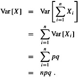 |
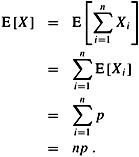
As can be seen from Figure C.2, the binomial distribution b(k; n, p) increases as k runs from 0 to n until it reaches the mean np, and then it decreases. We can prove that the distribution always behaves in this manner by looking at the ratio of successive terms:
This ratio is greater than 1 precisely when (n + 1) p - k is positive. Consequently, b(k; n, p) > b(k - 1; n, p) for k < (n + 1) p (the distribution increases), and b(k; n, p) < b(k - 1; n, p) for k > (n + 1) p (the distribution decreases). If k = (n + 1) p is an integer, then b(k; n, p) = b(k - 1; n, p), so the distribution has two maxima: at k = (n + 1) p and at k - 1 = (n + 1) p - 1 = np - q. Otherwise, it attains a maximum at the unique integer k that lies in the range np - q < k < (n + 1) p.
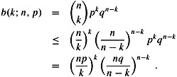
The following lemma provides an upper bound on the binomial distribution.
Let n ≥ 0, let 0 < p < 1, let q = 1 - p, and let 0 ≤ k ≤ n. Then
Proof Using equation (C.6), we have
How many times on average must we flip 6 fair coins before we obtain 3 heads and 3 tails?
Show that value of the maximum of the binomial distribution b(k; n, p) is approximately ![]() , where q = 1 - p.
, where q = 1 - p.
Show that the probability of no successes in n Bernoulli trials, each with probability p = 1/n, is approximately 1/e. Show that the probability of exactly one success is also approximately 1/e.
Professor Rosencrantz flips a fair coin n times, and so does Professor Guildenstern. Show that the probability that they get the same number of heads is ![]() . (Hint: For Professor Rosencrantz, call a head a success; for Professor Guildenstern, call a tail a success.) Use your argument to verify the identity
. (Hint: For Professor Rosencrantz, call a head a success; for Professor Guildenstern, call a tail a success.) Use your argument to verify the identity
Consider n Bernoulli trials, where for i = 1, 2,..., n, the ith trial has probability pi of success, and let X be the random variable denoting the total number of successes. Let p ≥ pi for all i = 1, 2,..., n. Prove that for 1 ≤ k ≤ n,
Let X be the random variable for the total number of successes in a set A of n Bernoulli trials, where the ith trial has a probability pi of success, and let X' be the random variable for the total number of successes in a second set A' of n Bernoulli trials, where the ith trial has a probability ![]() of success. Prove that for 0 ≤ k ≤ n,
of success. Prove that for 0 ≤ k ≤ n,
Pr {X' ≥ k} ≥ Pr{X ≥ k}.
(Hint: Show how to obtain the Bernoulli trials in A' by an experiment involving the trials of A, and use the result of Exercise C.3-7.)
|
|
< Day Day Up > |
|