|
|
< Day Day Up > |
|
Like the other basic operations on an n-node red-black tree, deletion of a node takes time O(lg n). Deleting a node from a red-black tree is only slightly more complicated than inserting a node.
The procedure RB-DELETE is a minor modification of the TREE-DELETE procedure (Section 12.3). After splicing out a node, it calls an auxiliary procedure RB-DELETE-FIXUP that changes colors and performs rotations to restore the red-black properties.
RB-DELETE(T, z)
 1 if left[z] = nil[T] or right[z] = nil[T]
 2    then y ← z
 3    else y ← TREE-SUCCESSOR(z)
 4 if left[y] ≠ nil[T]
 5    then x ← left[y]
 6    else x ← right[y]
 7 p[x] ← p[y]
 8 if p[y] = nil[T]
 9    then root[T] ← x
10    else if y = left[p[y]]
11            then left[p[y]] ← x
12            else right[p[y]] ← x
13 if y 3≠ z
14    then key[z] ← key[y]
15         copy y's satellite data into z
16 if color[y] = BLACK
17    then RB-DELETE-FIXUP(T, x)
18 return y
There are three differences between the procedures TREE-DELETE and RB-DELETE. First, all references to NIL in TREE-DELETE are replaced by references to the sentinel nil[T ] in RB-DELETE. Second, the test for whether x is NIL in line 7 of TREE-DELETE is removed, and the assignment p[x] ← p[y] is performed unconditionally in line 7 of RB-DELETE. Thus, if x is the sentinel nil[T], its parent pointer points to the parent of the spliced-out node y. Third, a call to RB-DELETE-FIXUP is made in lines 16-17 if y is black. If y is red, the red-black properties still hold when y is spliced out, for the following reasons:
no black-heights in the tree have changed,
no red nodes have been made adjacent, and
since y could not have been the root if it was red, the root remains black.
The node x passed to RB-DELETE-FIXUP is one of two nodes: either the node that was y's sole child before y was spliced out if y had a child that was not the sentinel nil[T ], or, if y had no children, x is the sentinel nil[T ]. In the latter case, the unconditional assignment in line 7 guarantees that x's parent is now the node that was previously y's parent, whether x is a key-bearing internal node or the sentinel nil[T].
We can now examine how the procedure RB-DELETE-FIXUP restores the red-black properties to the search tree.
RB-DELETE-FIXUP(T, x)
 1 while x ≠ root[T] and color[x] = BLACK
 2     do if x = left[p[x]]
 3           then w ← right[p[x]]
 4                if color[w] = RED
 5                   then color[w] ← BLACK                        ▹  Case 1
 6                        color[p[x]] ← RED                       ▹  Case 1
 7                        LEFT-ROTATE(T, p[x])                    ▹  Case 1
 8                        w ← right[p[x]]                         ▹  Case 1
 9                if color[left[w]] = BLACK and color[right[w]] = BLACK
10                   then color[w] ← RED                          ▹  Case 2
11                        x p[x]                                  ▹  Case 2
12                   else if color[right[w]] = BLACK
13                           then color[left[w]] ← BLACK          ▹  Case 3
14                                color[w] ← RED                  ▹  Case 3
15                                RIGHT-ROTATE(T, w)              ▹  Case 3
16                                w ← right[p[x]]                 ▹  Case 3
17                         color[w] ← color[p[x]]                 ▹  Case 4
18                         color[p[x]] ← BLACK                    ▹  Case 4
19                         color[right[w]] ← BLACK                ▹  Case 4
20                         LEFT-ROTATE(T, p[x])                   ▹  Case 4
21                         x ← root[T]                            ▹  Case 4
22        else (same as then clause with "right" and "left" exchanged)
23 color[x] ← BLACK
If the spliced-out node y in RB-DELETE is black, three problems may arise. First, if y had been the root and a red child of y becomes the new root, we have violated property 2. Second, if both x and p[y] (which is now also p[x]) were red, then we have violated property 4. Third, y's removal causes any path that previously contained y to have one fewer black node. Thus, property 5 is now violated by any ancestor of y in the tree. We can correct this problem by saying that node x has an "extra" black. That is, if we add 1 to the count of black nodes on any path that contains x, then under this interpretation, property 5 holds. When we splice out the black node y, we "push" its blackness onto its child. The problem is that now node x is neither red nor black, thereby violating property 1. Instead, node x is either "doubly black" or "red-and-black," and it contributes either 2 or 1, respectively, to the count of black nodes on paths containing x. The color attribute of x will still be either RED (if x is red-and-black) or BLACK (if x is doubly black). In other words, the extra black on a node is reflected in x's pointing to the node rather than in the color attribute.
The procedure RB-DELETE-FIXUP restores properties 1, 2, and 4. Exercises 13.4-1 and 13.4-2 ask you to show that the procedure restores properties 2 and 4, and so in the remainder of this section, we shall focus on property 1. The goal of the while loop in lines 1-22 is to move the extra black up the tree until
x points to a red-and-black node, in which case we color x (singly) black in line 23,
x points to the root, in which case the extra black can be simply "removed," or
suitable rotations and recolorings can be performed.
Within the while loop, x always points to a nonroot doubly black node. We determine in line 2 whether x is a left child or a right child of its parent p[x]. (We have given the code for the situation in which x is a left child; the situation in which x is a right child-line 22-is symmetric.) We maintain a pointer w to the sibling of x. Since node x is doubly black, node w cannot be nil[T]; otherwise, the number of blacks on the path from p[x] to the (singly black) leaf w would be smaller than the number on the path from p[x] to x.
The four cases[2] in the code are illustrated in Figure 13.7. Before examining each case in detail, let's look more generally at how we can verify that the transformation in each of the cases preserves property 5. The key idea is that in each case the number of black nodes (including x's extra black) from (and including) the root of the subtree shown to each of the subtrees α, β, ..., ζ is preserved by the transformation. Thus, if property 5 holds prior to the transformation, it continues to hold afterward. For example, in Figure 13.7(a), which illustrates case 1, the number of black nodes from the root to either subtree α or β is 3, both before and after the transformation. (Again, remember that node x adds an extra black.) Similarly, the number of black nodes from the root to any of γ, δ, ε, and is ζ, both before and after the transformation. In Figure 13.7(b), the counting must involve the value c of the color attribute of the root of the subtree shown, which can be either RED or BLACK. If we define count(RED) = 0 and count(BLACK) = 1, then the number of black nodes from the root to α is 2 + count(c), both before and after the transformation. In this case, after the transformation, the new node x has color attribute c, but this node is really either red-and-black (if c = RED) or doubly black (if c = BLACK). The other cases can be verified similarly (see Exercise 13.4-5).
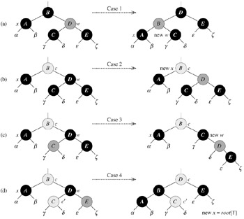
Case 1 (lines 5-8 of RB-DELETE-FIXUP and Figure 13.7(a)) occurs when node w, the sibling of node x, is red. Since w must have black children, we can switch the colors of w and p[x] and then perform a left-rotation on p[x] without violating any of the red-black properties. The new sibling of x, which is one of w's children prior to the rotation, is now black, and thus we have converted case 1 into case 2, 3, or 4.
Cases 2, 3, and 4 occur when node w is black; they are distinguished by the colors of w's children.
In case 2 (lines 10-11 of RB-DELETE-FIXUP and Figure 13.7(b)), both of w's children are black. Since w is also black, we take one black off both x and w, leaving x with only one black and leaving w red. To compensate for removing one black from x and w, we would like to add an extra black to p[x], which was originally either red or black. We do so by repeating the while loop with p[x] as the new node x. Observe that if we enter case 2 through case 1, the new node x is red-and-black, since the original p[x] was red. Hence, the value c of the color attribute of the new node x is RED, and the loop terminates when it tests the loop condition. The new node x is then colored (singly) black in line 23.
Case 3 (lines 13-16 and Figure 13.7(c)) occurs when w is black, its left child is red, and its right child is black. We can switch the colors of w and its left child left[w] and then perform a right rotation on w without violating any of the red-black properties. The new sibling w of x is now a black node with a red right child, and thus we have transformed case 3 into case 4.
Case 4 (lines 17-21 and Figure 13.7(d)) occurs when node x's sibling w is black and w's right child is red. By making some color changes and performing a left rotation on p[x], we can remove the extra black on x, making it singly black, without violating any of the red-black properties. Setting x to be the root causes the while loop to terminate when it tests the loop condition.
What is the running time of RB-DELETE? Since the height of a red-black tree of n nodes is O(lg n), the total cost of the procedure without the call to RB-DELETE-FIXUP takes O(lg n) time. Within RB-DELETE-FIXUP, cases 1, 3, and 4 each terminate after performing a constant number of color changes and at most three rotations. Case 2 is the only case in which the while loop can be repeated, and then the pointer x moves up the tree at most O(lg n) times and no rotations are performed. Thus, the procedure RB-DELETE-FIXUP takes O(lg n) time and performs at most three rotations, and the overall time for RB-DELETE is therefore also O(lg n).
Argue that if in RB-DELETE both x and p[y] are red, then property 4 is restored by the call RB-DELETE-FIXUP(T, x).
In Exercise 13.3-2, you found the red-black tree that results from successively inserting the keys 41, 38, 31, 12, 19, 8 into an initially empty tree. Now show the red-black trees that result from the successive deletion of the keys in the order 8, 12, 19, 31, 38, 41.
In which lines of the code for RB-DELETE-FIXUP might we examine or modify the sentinel nil[T]?
In each of the cases of Figure 13.7, give the count of black nodes from the root of the subtree shown to each of the subtrees α, β, ..., ζ, and verify that each count remains the same after the transformation. When a node has a color attribute c or c′, use the notation count(c) or count(c′) symbolically in your count.
Professors Skelton and Baron are concerned that at the start of case 1 of RB-DELETE-FIXUP, the node p[x] might not be black. If the professors are correct, then lines 5-6 are wrong. Show that p[x] must be black at the start of case 1, so that the professors have nothing to worry about.
Suppose that a node x is inserted into a red-black tree with RB-INSERT and then immediately deleted with RB-DELETE. Is the resulting red-black tree the same as the initial red-black tree? Justify your answer.
During the course of an algorithm, we sometimes find that we need to maintain past versions of a dynamic set as it is updated. Such a set is called persistent. One way to implement a persistent set is to copy the entire set whenever it is modified, but this approach can slow down a program and also consume much space. Sometimes, we can do much better.
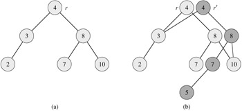
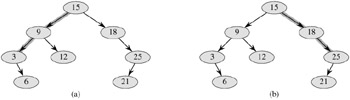
Consider a persistent set S with the operations INSERT, DELETE, and SEARCH, which we implement using binary search trees as shown in Figure 13.8(a). We maintain a separate root for every version of the set. In order to insert the key 5 into the set, we create a new node with key 5. This node becomes the left child of a new node with key 7, since we cannot modify the existing node with key 7. Similarly, the new node with key 7 becomes the left child of a new node with key 8 whose right child is the existing node with key 10. The new node with key 8 becomes, in turn, the right child of a new root r′ with key 4 whose left child is the existing node with key 3. We thus copy only part of the tree and share some of the nodes with the original tree, as shown in Figure 13.8(b).
Assume that each tree node has the fields key, left, and right but no parent field. (See also Exercise 13.3-6.)
For a general persistent binary search tree, identify the nodes that need to be changed to insert a key k or delete a node y.
Write a procedure PERSISTENT-TREE-INSERT that, given a persistent tree T and a key k to insert, returns a new persistent tree T′ that is the result of inserting k into T.
If the height of the persistent binary search tree T is h, what are the time and space requirements of your implementation of PERSISTENT-TREE-INSERT? (The space requirement is proportional to the number of new nodes allocated.)
Suppose that we had included the parent field in each node. In this case, PERSISTENT-TREE-INSERT would need to perform additional copying. Prove that PERSISTENT-TREE-INSERT would then require Ω(n) time and space, where n is the number of nodes in the tree.
Show how to use red-black trees to guarantee that the worst-case running time and space are O(lg n) per insertion or deletion.
The join operation takes two dynamic sets S1 and S2 and an element x such that for any x1 ∈ S1 and x2 ∈ S2, we have key[x1] ≤ key[x] ≤ key[x2]. It returns a set S = S1 ∪ {x} ∪ S2. In this problem, we investigate how to implement the join operation on red-black trees.
Given a red-black tree T, we store its black-height as the field bh[T]. Argue that this field can be maintained by RB-INSERT and RB-DELETE without requiring extra storage in the nodes of the tree and without increasing the asymptotic running times. Show that while descending through T, we can determine the black-height of each node we visit in O(1) time per node visited.
We wish to implement the operation RB-JOIN(T1, x, T2), which destroys T1 and T2 and returns a red-black tree T = T1 ∪ {x} ∪ T2. Let n be the total number of nodes in T1 and T2.
Assume that bh[T1] ≥ bh[T2]. Describe an O(lg n)-time algorithm that finds a black node y in T1 with the largest key from among those nodes whose black-height is bh[T2].
Let Ty be the subtree rooted at y. Describe how Ty ∪ {x} ∪ T2 can replace Ty in O(1) time without destroying the binary-search-tree property.
What color should we make x so that red-black properties 1, 3, and 5 are maintained? Describe how properties 2 and 4 can be enforced in O(lg n) time.
Argue that no generality is lost by making the assumption in part (b). Describe the symmetric situation that arises when bh[T1] = bh[T2].
Argue that the running time of RB-JOIN is O(lg n).
An AVL tree is a binary search tree that is height balanced: for each node x, the heights of the left and right subtrees of x differ by at most 1. To implement an AVL tree, we maintain an extra field in each node: h[x] is the height of node x. As for any other binary search tree T, we assume that root[T] points to the root node.
Prove that an AVL tree with n nodes has height O(lg n). (Hint: Prove that in an AVL tree of height h, there are at least Fh nodes, where Fh is the hth Fibonacci number.)
To insert into an AVL tree, a node is first placed in the appropriate place in binary search tree order. After this insertion, the tree may no longer be height balanced. Specifically, the heights of the left and right children of some node may differ by 2. Describe a procedure BALANCE(x), which takes a subtree rooted at x whose left and right children are height balanced and have heights that differ by at most 2, i.e., |h[right[x]] - h[left[x]]| ≤ 2, and alters the subtree rooted at x to be height balanced. (Hint: Use rotations.)
Using part (b), describe a recursive procedure AVL-INSERT(x, z), which takes a node x within an AVL tree and a newly created node z (whose key has already been filled in), and adds z to the subtree rooted at x, maintaining the property that x is the root of an AVL tree. As in TREE-INSERT from Section 12.3, assume that key[z] has already been filled in and that left[z] = NIL and right[z] = NIL; also assume that h[z] = 0. Thus, to insert the node z into the AVL tree T, we call AVL-INSERT(root[T], z).
Give an example of an n-node AVL tree in which an AVL-INSERT operation causes Ω(lg n) rotations to be performed.
If we insert a set of n items into a binary search tree, the resulting tree may be horribly unbalanced, leading to long search times. As we saw in Section 12.4, however, randomly built binary search trees tend to be balanced. Therefore, a strategy that, on average, builds a balanced tree for a fixed set of items is to randomly permute the items and then insert them in that order into the tree.
What if we do not have all the items at once? If we receive the items one at a time, can we still randomly build a binary search tree out of them?
We will examine a data structure that answers this question in the affirmative. A treap is a binary search tree with a modified way of ordering the nodes. Figure 13.9 shows an example. As usual, each node x in the tree has a key value key[x]. In addition, we assign priority[x], which is a random number chosen independently for each node. We assume that all priorities are distinct and also that all keys are distinct. The nodes of the treap are ordered so that the keys obey the binary-search-tree property and the priorities obey the min-heap order property:
If v is a left child of u, then key[v] < key[u].
If v is a right child of u, then key[v] > key[u].
If v is a child of u, then priority[v] > priority[u].
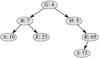
(This combination of properties is why the tree is called a "treap;" it has features of both a binary search tree and a heap.)
It helps to think of treaps in the following way. Suppose that we insert nodes x1, x2, ..., xn, with associated keys, into a treap. Then the resulting treap is the tree that would have been formed if the nodes had been inserted into a normal binary search tree in the order given by their (randomly chosen) priorities, i.e., priority[xi] < priority[xj] means that xi was inserted before xj.
Show that given a set of nodes x1, x2, ..., xn, with associated keys and priorities (all distinct), there is a unique treap associated with these nodes.
Show that the expected height of a treap is Θ(lg n), and hence the time to search for a value in the treap is Θ(lg n).
Let us see how to insert a new node into an existing treap. The first thing we do is assign to the new node a random priority. Then we call the insertion algorithm, which we call TREAP-INSERT, whose operation is illustrated in Figure 13.10.
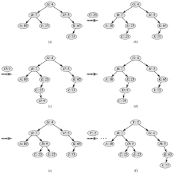
Explain how TREAP-INSERT works. Explain the idea in English and give pseudocode. (Hint: Execute the usual binary-search-tree insertion procedure and then perform rotations to restore the min-heap order property.)
Show that the expected running time of TREAP-INSERT is Θ(lg n).
TREAP-INSERT performs a search and then a sequence of rotations. Although these two operations have the same expected running time, they have different costs in practice. A search reads information from the treap without modifying it. In contrast, a rotation changes parent and child pointers within the treap. On most computers, read operations are much faster than write operations. Thus we would like TREAP-INSERT to perform few rotations. We will show that the expected number of rotations performed is bounded by a constant.
In order to do so, we will need some definitions, which are illustrated in Figure 13.11. The left spine of a binary search tree T is the path from the root to the node with the smallest key. In other words, the left spine is the path from the root that consists of only left edges. Symmetrically, the right spine of T is the path from the root consisting of only right edges. The length of a spine is the number of nodes it contains.
Consider the treap T immediately after x is inserted using TREAP-INSERT. Let C be the length of the right spine of the left subtree of x. Let D be the length of the left spine of the right subtree of x. Prove that the total number of rotations that were performed during the insertion of x is equal to C + D.
We will now calculate the expected values of C and D. Without loss of generality, we assume that the keys are 1, 2, ..., n, since we are comparing them only to one another.
For nodes x and y, where y ≠ x, let k = key[x] and i = key[y]. We define indicator random variables
Xi,k = I {y is in the right spine of the left subtree of x (in T)}.
Show that Xi,k = 1 if and only if priority[y] > priority[x], key[y] < key[x], and, for every z such that key[y] < key[z] < key[x], we have priority[y] < priority[z].
Show that
Show that
Use a symmetry argument to show that
Conclude that the expected number of rotations performed when inserting a node into a treap is less than 2.
[2]As in RB-INSERT-FIXUP, the cases in RB-DELETE-FIXUP are not mutually exclusive.
|
|
< Day Day Up > |
|