Counting the number of parenthesizations

Before solving the matrix-chain multiplication problem by dynamic programming, let us convince ourselves that exhaustively checking all possible parenthesizations does not yield an efficient algorithm. Denote the number of alternative parenthesizations of a sequence of n matrices by P(n). When n = 1, there is just one matrix and therefore only one way to fully parenthesize the matrix product. When n ≥ 2, a fully parenthesized matrix product is the product of two fully parenthesized matrix subproducts, and the split between the two subproducts may occur between the kth and (k + 1)st matrices for any k = 1, 2, ..., n - 1. Thus, we obtain the recurrence

(15.11)

Problem 12-4 asked you to show that the solution to a similar recurrence is the sequence of Catalan numbers, which grows as Ω(4ⁿ/n^3/2). A simpler exercise (see Exercise 15.2-3) is to show that the solution to the recurrence (15.11) is Ω(2ⁿ). The number of solutions is thus exponential in n, and the brute-force method of exhaustive search is therefore a poor strategy for determining the optimal parenthesization of a matrix chain.

Step 1: The structure of an optimal parenthesization

Our first step in the dynamic-programming paradigm is to find the optimal substructure and then use it to construct an optimal solution to the problem from optimal solutions to subproblems. For the matrix-chain multiplication problem, we can perform this step as follows. For convenience, let us adopt the notation A_i‥j, where i ≤ j, for the matrix that results from evaluating the product A_i A_i+1 A_j. Observe that if the problem is nontrivial, i.e., i < j, then any parenthesization of the product A_i A_i+1 A_j must split the product between A_k and A_k+1 for some integer k in the range i ≤ k < j. That is, for some value of k, we first compute the matrices A_i‥k and A_k+1‥j and then multiply them together to produce the final product A_i‥j. The cost of this parenthesization is thus the cost of computing the matrix A_i‥k, plus the cost of computing A_k+1‥j, plus the cost of multiplying them together.

The optimal substructure of this problem is as follows. Suppose that an optimal parenthesization of A_i A_i+1 A_j splits the product between A_k and A_k+1. Then the parenthesization of the "prefix" subchain A_i A_i+1 A_k within this optimal parenthesization of A_i A_i+1 A_j must be an optimal parenthesization of A_i A_i+1 A_k. Why? If there were a less costly way to parenthesize A_i A_i+1 A_k, substituting that parenthesization in the optimal parenthesization of A_i A_i+1 A_j would produce another parenthesization of A_i A_i+1 A_j whose cost was lower than the optimum: a contradiction. A similar observation holds for the parenthesization of the subchain A_k+1 A_k+2 A_j in the optimal parenthesization of A_i A_i+1 A_j: it must be an optimal parenthesization of A_k+1 A_k+2 A_j.

Now we use our optimal substructure to show that we can construct an optimal solution to the problem from optimal solutions to subproblems. We have seen that any solution to a nontrivial instance of the matrix-chain multiplication problem requires us to split the product, and that any optimal solution contains within it optimal solutions to subproblem instances. Thus, we can build an optimal solution to an instance of the matrix-chain multiplication problem by splitting the problem into two subproblems (optimally parenthesizing A_i A_i+1 A_k and A_k+1 A_k+2 A_j), finding optimal solutions to subproblem instances, and then combining these optimal subproblem solutions. We must ensure that when we search for the correct place to split the product, we have considered all possible places so that we are sure of having examined the optimal one.

Step 2: A recursive solution

Next, we define the cost of an optimal solution recursively in terms of the optimal solutions to subproblems. For the matrix-chain multiplication problem, we pick as our subproblems the problems of determining the minimum cost of a parenthesization of A_i A_i+1 A_j for 1 ≤ i ≤ j ≤ n. Let m[i, j] be the minimum number of scalar multiplications needed to compute the matrix A_i‥j; for the full problem, the cost of a cheapest way to compute A_1‥n would thus be m[1, n].

We can define m[i, j] recursively as follows. If i = j, the problem is trivial; the chain consists of just one matrix A_i‥i = A_i, so that no scalar multiplications are necessary to compute the product. Thus, m[i, i] = 0 for i = 1, 2, ..., n. To compute m[i, j] when i < j, we take advantage of the structure of an optimal solution from step 1. Let us assume that the optimal parenthesization splits the product A_i A_i+1 A_j between A_k and A_k+1, where i ≤ k < j. Then, m[i, j] is equal to the minimum cost for computing the subproducts A_i‥k and A_k+1‥j, plus the cost of multiplying these two matrices together. Recalling that each matrix A_i is p_i-1 × p_i, we see that computing the matrix product A_i‥k A_k+1‥j takes p_i-1 p_k p_j scalar multiplications. Thus, we obtain

m[i, j ] = m[i, k] + m[k + 1, j ] + p_i-1 p_k p_j.

This recursive equation assumes that we know the value of k, which we do not. There are only j - i possible values for k, however, namely k = i, i + 1, ..., j - 1. Since the optimal parenthesization must use one of these values for k, we need only check them all to find the best. Thus, our recursive definition for the minimum cost of parenthesizing the product A_i A_i+1 A_j becomes

(15.12)

The m[i, j] values give the costs of optimal solutions to subproblems. To help us keep track of how to construct an optimal solution, let us define s[i, j] to be a value of k at which we can split the product A_i A_i+1 A_j to obtain an optimal parenthesization. That is, s[i, j] equals a value k such that m[i, j] = m[i, k] + m[k + 1, j] + p_i-1 p_k p_j.

Step 3: Computing the optimal costs

At this point, it is a simple matter to write a recursive algorithm based on recurrence (15.12) to compute the minimum cost m[1, n] for multiplying A₁ A₂ A_n. As we shall see in Section 15.3, however, this algorithm takes exponential time, which is no better than the brute-force method of checking each way of parenthesizing the product.

The important observation that we can make at this point is that we have relatively few subproblems: one problem for each choice of i and j satisfying 1 ≤ i ≤ j ≤ n, or in all. A recursive algorithm may encounter each subproblem many times in different branches of its recursion tree. This property of overlapping subproblems is the second hallmark of the applicability of dynamic programming (the first hallmark being optimal substructure).

Instead of computing the solution to recurrence (15.12) recursively, we perform the third step of the dynamic-programming paradigm and compute the optimal cost by using a tabular, bottom-up approach. The following pseudocode assumes that matrix A_i has dimensions p_i-1 × p_i for i = 1, 2, ..., n. The input is a sequence p = 〈p₀, p₁, ..., p_n〉, where length[p] = n + 1. The procedure uses an auxiliary table m[1 ‥ n, 1 ‥ n] for storing the m[i, j] costs and an auxiliary table s[1 ‥ n, 1 ‥ n] that records which index of k achieved the optimal cost in computing m[i, j]. We will use the table s to construct an optimal solution.

In order to correctly implement the bottom-up approach, we must determine which entries of the table are used in computing m[i, j]. Equation (15.12) shows that the cost m[i, j] of computing a matrix-chain product of j - i + 1 matrices depends only on the costs of computing matrix-chain products of fewer than j - i + 1 matrices. That is, for k = i, i + 1, ..., j - 1, the matrix A_i‥k is a product of k - i + 1 < j - i + 1 matrices and the matrix A_k+1‥j is a product of j - k < j - i + 1 matrices. Thus, the algorithm should fill in the table m in a manner that corresponds to solving the parenthesization problem on matrix chains of increasing length.

MATRIX-CHAIN-ORDER(p)
 1 n ← length[p] - 1
 2 for i ← 1 to n
 3      do m[i, i] ← 0
 4 for l ← 2 to n      ▹l is the chain length.
 5      do for i ← 1 to n - l + 1
 6             do j ← i + l - 1
 7                m[i, j] ← ∞
 8                for k ← i to j - 1
 9                    do q ← m[i, k] + m[k + 1, j] + pi-1 pkpj
10                       if q < m[i, j]
11                          then m[i, j] ← q
12                               s[i, j] ← k
13 return m and s

The algorithm first computes m[i, i] ← 0 for i = 1, 2, ..., n (the minimum costs for chains of length 1) in lines 2-3. It then uses recurrence (15.12) to compute m[i, i + 1] for i = 1, 2, ..., n - 1 (the minimum costs for chains of length l = 2) during the first execution of the loop in lines 4-12. The second time through the loop, it computes m[i, i + 2] for i = 1, 2, ..., n - 2 (the minimum costs for chains of length l = 3), and so forth. At each step, the m[i, j] cost computed in lines 9-12 depends only on table entries m[i, k] and m[k + 1, j] already computed.

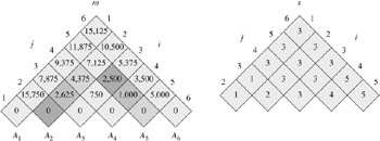
Figure 15.3 illustrates this procedure on a chain of n = 6 matrices. Since we have defined m[i, j] only for i ≤ j, only the portion of the table m strictly above the main diagonal is used. The figure shows the table rotated to make the main diagonal run horizontally. The matrix chain is listed along the bottom. Using this layout, the minimum cost m[i, j] for multiplying a subchain A_i A_i+1 A_j of matrices can be found at the intersection of lines running northeast from A_i and northwest from A_j. Each horizontal row in the table contains the entries for matrix chains of the same length. MATRIX-CHAIN-ORDER computes the rows from bottom to top and from left to right within each row. An entry m[i, j] is computed using the products p_i-1 p_k p_j for k = i, i + 1, ..., j - 1 and all entries southwest and southeast from m[i, j].

Figure 15.3: The m and s tables computed by MATRIX-CHAIN-ORDER for n = 6 and the following matrix dimensions:

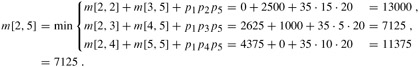
The tables are rotated so that the main diagonal runs horizontally. Only the main diagonal and upper triangle are used in the m table, and only the upper triangle is used in the s table. The minimum number of scalar multiplications to multiply the 6 matrices is m[1, 6] = 15,125. Of the darker entries, the pairs that have the same shading are taken together in line 9 when computing

A simple inspection of the nested loop structure of MATRIX-CHAIN-ORDER yields a running time of O(n³) for the algorithm. The loops are nested three deep, and each loop index (l, i, and k) takes on at most n -1 values. Exercise 15.2-4 asks you to show that the running time of this algorithm is in fact also Ω(n³). The algorithm requires Θ(n²) space to store the m and s tables. Thus, MATRIX-CHAIN-ORDER is much more efficient than the exponential-time method of enumerating all possible parenthesizations and checking each one.

Step 4: Constructing an optimal solution

Although MATRIX-CHAIN-ORDER determines the optimal number of scalar multiplications needed to compute a matrix-chain product, it does not directly show how to multiply the matrices. It is not difficult to construct an optimal solution from the computed information stored in the table s[1 ‥ n, 1 ‥ n]. Each entry s[i, j] records the value of k such that the optimal parenthesization of A_i A_i+1 ··· A_j splits the product between A_k and A_k+1. Thus, we know that the final matrix multiplication in computing A_1‥n optimally is A_1‥s[1,n] A_s[1,n]+1‥n. The earlier matrix multiplications can be computed recursively, since s[1, s[1, n]] determines the last matrix multiplication in computing A_1‥s[1,n], and s[s[1, n] + 1, n] determines the last matrix multiplication in computing A_s[1,n]+1‥n. The following recursive procedure prints an optimal parenthesization of 〈A_i, A_i+1, ..., A_j〉, given the s table computed by MATRIX-CHAIN-ORDER and the indices i and j. The initial call PRINT-OPTIMAL-PARENS(s, 1, n) prints an optimal parenthesization of 〈A₁, A₂, ..., A_n〉.

PRINT-OPTIMAL-PARENS(s, i, j)
1 if i = j
2     then print "A"i
3     else print "("
4          PRINT-OPTIMAL-PARENS(s, i, s[i, j])
5          PRINT-OPTIMAL-PARENS(s, s[i, j] + 1, j)
6          print ")"

In the example of Figure 15.3, the call PRINT-OPTIMAL-PARENS(s, 1, 6) prints the parenthesization ((A₁ (A₂ A₃)) ((A₄ A₅)A₆)).

Exercises 15.2-1

Find an optimal parenthesization of a matrix-chain product whose sequence of dimensions is 〈5, 10, 3, 12, 5, 50, 6〉.

Exercises 15.2-2

Give a recursive algorithm MATRIX-CHAIN-MULTIPLY(A, s, i, j) that actually performs the optimal matrix-chain multiplication, given the sequence of matrices 〈A₁, A₂, ..., A_n〉, the s table computed by MATRIX-CHAIN-ORDER, and the indices i and j. (The initial call would be MATRIX-CHAIN-MULTIPLY(A, s, 1, n).)

Exercises 15.2-3

Use the substitution method to show that the solution to the recurrence (15.11) is Ω(2ⁿ).

Exercises 15.2-4

Let R(i, j) be the number of times that table entry m[i, j] is referenced while computing other table entries in a call of MATRIX-CHAIN-ORDER. Show that the total number of references for the entire table is

(Hint: You may find equation (A.3) useful.)

Exercises 15.2-5

Show that a full parenthesization of an n-element expression has exactly n - 1 pairs of parentheses.