Optimal substructure

The first step in solving an optimization problem by dynamic programming is to characterize the structure of an optimal solution. Recall that a problem exhibits optimal substructure if an optimal solution to the problem contains within it optimal solutions to subproblems. Whenever a problem exhibits optimal substructure, it is a good clue that dynamic programming might apply. (It also might mean that a greedy strategy applies, however. See Chapter 16.) In dynamic programming, we build an optimal solution to the problem from optimal solutions to subproblems. Consequently, we must take care to ensure that the range of subproblems we consider includes those used in an optimal solution.

We discovered optimal substructure in both of the problems we have examined in this chapter so far. In Section 15.1, we observed that the fastest way through station j of either line contained within it the fastest way through station j - 1 on one line. In Section 15.2, we observed that an optimal parenthesization of A_i A_i+1 A_j that splits the product between A_k and A_k+1 contains within it optimal solutions to the problems of parenthesizing A_i A_i+1 A_k and A_k+1 A_k+2 A_j.

You will find yourself following a common pattern in discovering optimal substructure:

1. You show that a solution to the problem consists of making a choice, such as choosing a preceding assembly-line station or choosing an index at which to split the matrix chain. Making this choice leaves one or more subproblems to be solved.

2. You suppose that for a given problem, you are given the choice that leads to an optimal solution. You do not concern yourself yet with how to determine this choice. You just assume that it has been given to you.

3. Given this choice, you determine which subproblems ensue and how to best characterize the resulting space of subproblems.

4. You show that the solutions to the subproblems used within the optimal solution to the problem must themselves be optimal by using a "cut-and-paste" technique. You do so by supposing that each of the subproblem solutions is not optimal and then deriving a contradiction. In particular, by "cutting out" the nonoptimal subproblem solution and "pasting in" the optimal one, you show that you can get a better solution to the original problem, thus contradicting your supposition that you already had an optimal solution. If there is more than one subproblem, they are typically so similar that the cut-and-paste argument for one can be modified for the others with little effort.

To characterize the space of subproblems, a good rule of thumb is to try to keep the space as simple as possible, and then to expand it as necessary. For example, the space of subproblems that we considered for assembly-line scheduling was the fastest way from entry into the factory through stations S_{1, j} and S_{2, j}. This subproblem space worked well, and there was no need to try a more general space of subproblems.

Conversely, suppose that we had tried to constrain our subproblem space for matrix-chain multiplication to matrix products of the form A₁ A₂ A_j. As before, an optimal parenthesization must split this product between A_k and A_k+1 for some 1 ≤ k ≤ j. Unless we could guarantee that k always equals j - 1, we would find that we had subproblems of the form A₁ A₂ A_k and A_k+1 A_k+2 A_j, and that the latter subproblem is not of the form A₁ A₂ A_j. For this problem, it was necessary to allow our subproblems to vary at "both ends," that is, to allow both i and j to vary in the subproblem A_i A_i+1 A_j.

Optimal substructure varies across problem domains in two ways:

1. how many subproblems are used in an optimal solution to the original problem, and

2. how many choices we have in determining which subproblem(s) to use in an optimal solution.

In assembly-line scheduling, an optimal solution uses just one subproblem, but we must consider two choices in order to determine an optimal solution. To find the fastest way through station S_i,j , we use either the fastest way through S₁, _{j -1} or the fastest way through S_{2, j -1}; whichever we use represents the one subproblem that we must optimally solve. Matrix-chain multiplication for the subchain A_i A_i+1 A_j serves as an example with two subproblems and j - i choices. For a given matrix A_k at which we split the product, we have two subproblems-parenthesizing A_i A_i+1 A_k and parenthesizing A_k+1 A_k+2 A_j-and we must solve both of them optimally. Once we determine the optimal solutions to subproblems, we choose from among j - i candidates for the index k.

Informally, the running time of a dynamic-programming algorithm depends on the product of two factors: the number of subproblems overall and how many choices we look at for each subproblem. In assembly-line scheduling, we had Θ(n) subproblems overall, and only two choices to examine for each, yielding a Θ(n) running time. For matrix-chain multiplication, there were Θ(n²) subproblems overall, and in each we had at most n - 1 choices, giving an O(n³) running time.

Dynamic programming uses optimal substructure in a bottom-up fashion. That is, we first find optimal solutions to subproblems and, having solved the subproblems, we find an optimal solution to the problem. Finding an optimal solution to the problem entails making a choice among subproblems as to which we will use in solving the problem. The cost of the problem solution is usually the subproblem costs plus a cost that is directly attributable to the choice itself. In assembly-line scheduling, for example, first we solved the subproblems of finding the fastest way through stations S_{1, j -1} and S_{2, j -1}, and then we chose one of these stations as the one preceding station S_{i, j}. The cost attributable to the choice itself depends on whether we switch lines between stations j - 1 and j; this cost is a_{i, j} if we stay on the same line, and it is t_{i′, j-1} + a_i,j , where i′ ≠ i, if we switch. In matrix-chain multiplication, we determined optimal parenthesizations of subchains of A_i A_i+1 A_j , and then we chose the matrix A_k at which to split the product. The cost attributable to the choice itself is the term p_i-1 p_k p_j.

In Chapter 16, we shall examine "greedy algorithms," which have many similarities to dynamic programming. In particular, problems to which greedy algorithms apply have optimal substructure. One salient difference between greedy algorithms and dynamic programming is that in greedy algorithms, we use optimal substructure in a top-down fashion. Instead of first finding optimal solutions to subproblems and then making a choice, greedy algorithms first make a choice-the choice that looks best at the time-and then solve a resulting subproblem.

Subtleties

One should be careful not to assume that optimal substructure applies when it does not. Consider the following two problems in which we are given a directed graph G = (V, E) and vertices u, v ∈ V.

• Unweighted shortest path: ^[2] Find a path from u to v consisting of the fewest edges. Such a path must be simple, since removing a cycle from a path produces a path with fewer edges.

• Unweighted longest simple path: Find a simple path from u to v consisting of the most edges. We need to include the requirement of simplicity because otherwise we can traverse a cycle as many times as we like to create paths with an arbitrarily large number of edges.

The unweighted shortest-path problem exhibits optimal substructure, as follows. Suppose that u ≠ v, so that the problem is nontrivial. Then any path p from u to v must contain an intermediate vertex, say w. (Note that w may be u or v.) Thus we can decompose the path into subpaths . Clearly, the number of edges in p is equal to the sum of the number of edges in p₁ and the number of edges in p₂. We claim that if p is an optimal (i.e., shortest) path from u to v, then p₁ must be a shortest path from u to w. Why? We use a "cut-and-paste" argument: if there were another path, say , from u to w with fewer edges than p₁, then we could cut out p₁ and paste in to produce a path with fewer edges than p, thus contradicting p's optimality. Symmetrically, p₂ must be a shortest path from w to v. Thus, we can find a shortest path from u to v by considering all intermediate vertices w, finding a shortest path from u to w and a shortest path from w to v, and choosing an intermediate vertex w that yields the overall shortest path. In Section 25.2, we use a variant of this observation of optimal substructure to find a shortest path between every pair of vertices on a weighted, directed graph.

It is tempting to assume that the problem of finding an unweighted longest simple path exhibits optimal substructure as well. After all, if we decompose a longest simple path into subpaths , then mustn't p₁ be a longest simple path from u to w, and mustn't p₂ be a longest simple path from w to v? The answer is no! Figure 15.4 gives an example. Consider the path q → r → t, which is a longest simple path from q to t. Is q → r a longest simple path from q to r? No, for the path q → s → t → r is a simple path that is longer. Is r → t a longest simple path from r to t? No again, for the path r → q → s → t is a simple path that is longer.

Figure 15.4: A directed graph showing that the problem of finding a longest simple path in an unweighted directed graph does not have optimal substructure. The path q → r → t is a longest simple path from q to t, but the subpath q → r is not a longest simple path from q to r, nor is the subpath r → t a longest simple path from r to t.

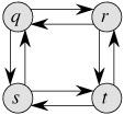
This example shows that for longest simple paths, not only is optimal substructure lacking, but we cannot necessarily assemble a "legal" solution to the problem from solutions to subproblems. If we combine the longest simple paths q → s → t → r and r → q → s → t, we get the path q → s → t → r → q → s → t, which is not simple. Indeed, the problem of finding an unweighted longest simple path does not appear to have any sort of optimal substructure. No efficient dynamic-programming algorithm for this problem has ever been found. In fact, this problem is NP-complete, which-as we shall see in Chapter 34-means that it is unlikely that it can be solved in polynomial time.

What is it about the substructure of a longest simple path that is so different from that of a shortest path? Although two subproblems are used in a solution to a problem for both longest and shortest paths, the subproblems in finding the longest simple path are not independent, whereas for shortest paths they are. What do we mean by subproblems being independent? We mean that the solution to one subproblem does not affect the solution to another subproblem of the same problem. For the example of Figure 15.4, we have the problem of finding a longest simple path from q to t with two subproblems: finding longest simple paths from q to r and from r to t. For the first of these subproblems, we choose the path q → s → t → r, and so we have also used the vertices s and t. We can no longer use these vertices in the second subproblem, since the combination of the two solutions to subproblems would yield a path that is not simple. If we cannot use vertex t in the second problem, then we cannot solve it all, since t is required to be on the path that we find, and it is not the vertex at which we are "splicing" together the subproblem solutions (that vertex being r). Our use of vertices s and t in one subproblem solution prevents them from being used in the other subproblem solution. We must use at least one of them to solve the other subproblem, however, and we must use both of them to solve it optimally. Thus we say that these subproblems are not independent. Looked at another way, our use of resources in solving one subproblem (those resources being vertices) has rendered them unavailable for the other subproblem.

Why, then, are the subproblems independent for finding a shortest path? The answer is that by nature, the subproblems do not share resources. We claim that if a vertex w is on a shortest path p from u to v, then we can splice together any shortest path and any shortest path to produce a shortest path from u to v. We are assured that, other than w, no vertex can appear in both paths p₁ and p₂. Why? Suppose that some vertex x ≠ w appears in both p₁ and p₂, so that we can decompose p₁ as and p₂ as . By the optimal substructure of this problem, path p has as many edges as p₁ and p₂ together; let's say that p has e edges. Now let us construct a path from u to v. This path has at most e - 2 edges, which contradicts the assumption that p is a shortest path. Thus, we are assured that the subproblems for the shortest-path problem are independent.

Both problems examined in Sections 15.1 and 15.2 have independent subproblems. In matrix-chain multiplication, the subproblems are multiplying subchains A_iA_i+1 A_k and A_k+1A_k+2 A_j. These subchains are disjoint, so that no matrix could possibly be included in both of them. In assembly-line scheduling, to determine the fastest way through station S_i,j, we look at the fastest ways through stations S_1,j-1 and S_2,j-1. Because our solution to the fastest way through station Si, j will include just one of these subproblem solutions, that subproblem is automatically independent of all others used in the solution.

Overlapping subproblems

The second ingredient that an optimization problem must have for dynamic programming to be applicable is that the space of subproblems must be "small" in the sense that a recursive algorithm for the problem solves the same subproblems over and over, rather than always generating new subproblems. Typically, the total number of distinct subproblems is a polynomial in the input size. When a recursive algorithm revisits the same problem over and over again, we say that the optimization problem has overlapping subproblems.^[3] In contrast, a problem for which a divide-and-conquer approach is suitable usually generates brand-new problems at each step of the recursion. Dynamic-programming algorithms typically take advantage of overlapping subproblems by solving each subproblem once and then storing the solution in a table where it can be looked up when needed, using constant time per lookup.

In Section 15.1, we briefly examined how a recursive solution to assembly-line scheduling makes 2^n-j references to f_i[j] for j = 1, 2, ..., n. Our tabular solution takes an exponential-time recursive algorithm down to linear time.

To illustrate the overlapping-subproblems property in greater detail, let us reexamine the matrix-chain multiplication problem. Referring back to Figure 15.3, observe that MATRIX-CHAIN-ORDER repeatedly looks up the solution to subproblems in lower rows when solving subproblems in higher rows. For example, entry m[3, 4] is referenced 4 times: during the computations of m[2, 4], m[1, 4], m[3, 5], and m[3, 6]. If m[3, 4] were recomputed each time, rather than just being looked up, the increase in running time would be dramatic. To see this, consider the following (inefficient) recursive procedure that determines m[i, j], the minimum number of scalar multiplications needed to compute the matrix-chain product A_i‥j = A_iA_i+1 ··· A_j. The procedure is based directly on the recurrence (15.12).

RECURSIVE-MATRIX-CHAIN(p, i, j)
1 if i = j
2     then return 0
3 m[i, j] ← ∞
4 for k ← i to j - 1
5      do q ← RECURSIVE-MATRIX-CHAIN(p, i, k)
                 + RECURSIVE-MATRIX-CHAIN(p,k + 1, j)
                 + pi-1 pk pj
6         if q < m[i, j]
7            then m[i, j] ← q
8 return m[i, j]

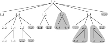
Figure 15.5 shows the recursion tree produced by the call RECURSIVE-MATRIX-CHAIN(p, 1, 4). Each node is labeled by the values of the parameters i and j. Observe that some pairs of values occur many times.

Figure 15.5: The recursion tree for the computation of RECURSIVE-MATRIX-CHAIN(p, 1, 4). Each node contains the parameters i and j. The computations performed in a shaded subtree are replaced by a single table lookup in MEMOIZED-MATRIX-CHAIN(p, 1, 4).

In fact, we can show that the time to compute m[1, n] by this recursive procedure is at least exponential in n. Let T (n) denote the time taken by RECURSIVE-MATRIX-CHAIN to compute an optimal parenthesization of a chain of n matrices. If we assume that the execution of lines 1-2 and of lines 6-7 each take at least unit time, then inspection of the procedure yields the recurrence

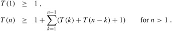
Noting that for i = 1, 2, ..., n - 1, each term T (i) appears once as T (k) and once as T (n - k), and collecting the n - 1 1's in the summation together with the 1 out front, we can rewrite the recurrence as

(15.13)

We shall prove that T (n) = Ω(2ⁿ) using the substitution method. Specifically, we shall show that T (n) ≥ 2^n-1 for all n ≥ 1. The basis is easy, since T (1) ≥ 1 = 2⁰. Inductively, for n ≥ 2 we have

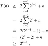
which completes the proof. Thus, the total amount of work performed by the call RECURSIVE-MATRIX-CHAIN(p, 1, n) is at least exponential in n.

Compare this top-down, recursive algorithm with the bottom-up, dynamic-programming algorithm. The latter is more efficient because it takes advantage of the overlapping-subproblems property. There are only Θ(n²) different subproblems, and the dynamic-programming algorithm solves each exactly once. The recursive algorithm, on the other hand, must repeatedly resolve each subproblem each time it reappears in the recursion tree. Whenever a recursion tree for the natural recursive solution to a problem contains the same subproblem repeatedly, and the total number of different subproblems is small, it is a good idea to see if dynamic programming can be made to work.

Reconstructing an optimal solution

As a practical matter, we often store which choice we made in each subproblem in a table so that we do not have to reconstruct this information from the costs that we stored. In assembly-line scheduling, we stored in l_i [j] the station preceding S_i,j in a fastest way through S_i,j . Alternatively, having filled in the entire f_i[j] table, we could determine which station precedes S_1,j in a fastest way through S_i,j with a little extra work. If f₁[j] = f₁[j - 1] + a_{1, j}, then station S_{1, j -1} precedes S_{1, j} in a fastest way through S_{1, j}. Otherwise, it must be the case that f₁[j] = f₂[j - 1] + t_{2, j -1} + a_{1, j}, and so S_{2, j - 1} precedes S_{1, j}. For assembly-line scheduling, reconstructing the predecessor stations takes only O(1) time per station, even without the l_i[j] table.

For matrix-chain multiplication, however, the table s[i, j] saves us a significant amount of work when reconstructing an optimal solution. Suppose that we did not maintain the s[i, j] table, having filled in only the table m[i, j] containing optimal subproblem costs. There are j - i choices in determining which subproblems to use in an optimal solution to parenthesizing A_i A_i+1 A_j, and j - i is not a constant. Therefore, it would take Θ(j - i) = ω(1) time to reconstruct which subproblems we chose for a solution to a given problem. By storing in s[i, j] the index of the matrix at which we split the product A_i A_i+1 A_j, we can reconstruct each choice in O(1) time.

Memoization

There is a variation of dynamic programming that often offers the efficiency of the usual dynamic-programming approach while maintaining a top-down strategy. The idea is to memoize the natural, but inefficient, recursive algorithm. As in ordinary dynamic programming, we maintain a table with subproblem solutions, but the control structure for filling in the table is more like the recursive algorithm.

A memoized recursive algorithm maintains an entry in a table for the solution to each subproblem. Each table entry initially contains a special value to indicate that the entry has yet to be filled in. When the subproblem is first encountered during the execution of the recursive algorithm, its solution is computed and then stored in the table. Each subsequent time that the subproblem is encountered, the value stored in the table is simply looked up and returned.^[4]

Here is a memoized version of RECURSIVE-MATRIX-CHAIN:

MEMOIZED-MATRIX-CHAIN(p)
1 n ← length[p] - 1
2 for i ← 1 to n
3      do for j ← i to n
4             do m[i, j] ← ∞
5 return LOOKUP-CHAIN(p, 1, n)

LOOKUP-CHAIN(p, i, j)
1 if m[i, j] < ∞
2    then return m[i, j]
3 if i = j
4     then m[i, j] ← 0
5     else for k ← i to j - 1
6             do q ← LOOKUP-CHAIN(p, i, k)
                        + LOOKUP-CHAIN(p,k + 1, j) + pi-1 pk pj
7                if q < m[i, j]
8                   then m[i, j] ← q
9 return m[i, j]

MEMOIZED-MATRIX-CHAIN, like MATRIX-CHAIN-ORDER, maintains a table m[1 ‥ n, 1 ‥ n] of computed values of m[i, j], the minimum number of scalar multiplications needed to compute the matrix A_i‥j. Each table entry initially contains the value ∞ to indicate that the entry has yet to be filled in. When the call LOOKUP-CHAIN(p, i, j) is executed, if m[i, j] < ∞ in line 1, the procedure simply returns the previously computed cost m[i, j] (line 2). Otherwise, the cost is computed as in RECURSIVE-MATRIX-CHAIN, stored in m[i, j], and returned. (The value ∞ is convenient to use for an unfilled table entry since it is the value used to initialize m[i, j] in line 3 of RECURSIVE-MATRIX-CHAIN.) Thus, LOOKUP-CHAIN(p, i, j) always returns the value of m[i, j], but it computes it only if this is the first time that LOOKUP-CHAIN has been called with the parameters i and j.

Figure 15.5 illustrates how MEMOIZED-MATRIX-CHAIN saves time compared to RECURSIVE-MATRIX-CHAIN. Shaded subtrees represent values that are looked up rather than computed.

Like the dynamic-programming algorithm MATRIX-CHAIN-ORDER, the procedure MEMOIZED-MATRIX-CHAIN runs in O(n³) time. Each of Θ(n²) table entries is initialized once in line 4 of MEMOIZED-MATRIX-CHAIN. We can categorize the calls of LOOKUP-CHAIN into two types:

1. calls in which m[i, j] = ∞, so that lines 3-9 are executed, and

2. calls in which m[i, j] < ∞, so that LOOKUP-CHAIN simply returns in line 2.

There are Θ(n²) calls of the first type, one per table entry. All calls of the second type are made as recursive calls by calls of the first type. Whenever a given call of LOOKUP-CHAIN makes recursive calls, it makes O(n) of them. Therefore, there are O(n³) calls of the second type in all. Each call of the second type takes O(1) time, and each call of the first type takes O(n) time plus the time spent in its recursive calls. The total time, therefore, is O(n³). Memoization thus turns an Ω(2ⁿ)-time algorithm into an O(n³)-time algorithm.

In summary, the matrix-chain multiplication problem can be solved by either a top-down, memoized algorithm or a bottom-up, dynamic-programming algorithm in O(n³) time. Both methods take advantage of the overlapping-subproblems property. There are only Θ(n²) different subproblems in total, and either of these methods computes the solution to each subproblem once. Without memoization, the natural recursive algorithm runs in exponential time, since solved subproblems are repeatedly solved.

In general practice, if all subproblems must be solved at least once, a bottom-up dynamic-programming algorithm usually outperforms a top-down memoized algorithm by a constant factor, because there is no overhead for recursion and less overhead for maintaining the table. Moreover, there are some problems for which the regular pattern of table accesses in the dynamic-programming algorithm can be exploited to reduce time or space requirements even further. Alternatively, if some subproblems in the subproblem space need not be solved at all, the memoized solution has the advantage of solving only those subproblems that are definitely required.

Exercises 15.3-1

Which is a more efficient way to determine the optimal number of multiplications in a matrix-chain multiplication problem: enumerating all the ways of parenthesizing the product and computing the number of multiplications for each, or running RECURSIVE-MATRIX-CHAIN? Justify your answer.

Exercises 15.3-2

Draw the recursion tree for the MERGE-SORT procedure from Section 2.3.1 on an array of 16 elements. Explain why memoization is ineffective in speeding up a good divide-and-conquer algorithm such as MERGE-SORT.

Exercises 15.3-3

Consider a variant of the matrix-chain multiplication problem in which the goal is to parenthesize the sequence of matrices so as to maximize, rather than minimize, the number of scalar multiplications. Does this problem exhibit optimal substructure?

Exercises 15.3-4

Describe how assembly-line scheduling has overlapping subproblems.

Exercises 15.3-5

As stated, in dynamic programming we first solve the subproblems and then choose which of them to use in an optimal solution to the problem. Professor Capulet claims that it is not always necessary to solve all the subproblems in order to find an optimal solution. She suggests that an optimal solution to the matrix-chain multiplication problem can be found by always choosing the matrix A_k at which to split the subproduct A_i A_i+1 A_j (by selecting k to minimize the quantity p_i-1 p_k p_j) before solving the subproblems. Find an instance of the matrix-chain multiplication problem for which this greedy approach yields a suboptimal solution.