The optimal substructure of the activity-selection problem

As mentioned above, we start by developing a dynamic-programming solution to the activity-selection problem. As in Chapter 15, our first step is to find the optimal substructure and then use it to construct an optimal solution to the problem from optimal solutions to subproblems.

We saw in Chapter 15 that we need to define an appropriate space of subproblems. Let us start by defining sets

S_ij = {a_k ∈ S : f_i ≤ s_k < f_k ≤ s_j} ,

so that S_ij is the subset of activities in S that can start after activity a_i finishes and finish before activity a_j starts. In fact, S_ij consists of all activities that are compatible with a_i and a_j and are also compatible with all activities that finish no later than a_i finishes and all activities that start no earlier than a_j starts. In order to represent to entire problem, we add fictitious activities a₀ and a_n+1 and adopt the conventions that f₀ = 0 and s_n+1 = ∞. Then S = S_0.n+1, and the ranges for i and j are given by 0 ≤ i, j ≤ n + 1.

We can further restrict the ranges of i and j as follows. Let us assume that the activities are sorted in monotonically increasing order of finish time:

(16.1)

We claim that S_ij = Ø whenever i ≥ j. Why? Suppose that there exists an activity a_k ∈ S_ij for some i ≥ j, so that a_i follows a_j in the sorted order. Then we would have f_i ≤ s_k < f_k ≤ s_j < f_j. Thus, f_i < f_j, which contradicts our assumption that a_i follows a_j in the sorted order. We can conclude that, assuming that we have sorted the activities in monotonically increasing order of finish time, our space of subproblems is to select a maximum-size subset of mutually compatible activities from S_ij, for 0 ≤ i < j ≤ n + 1, knowing that all other S_ij are empty.

To see the substructure of the activity-selection problem, consider some non-empty subproblem S_ij,^[1] and suppose that a solution to S_ij includes some activity a_k, so that f_i ≤ s_k < f_k ≤ s_j. Using activity a_k generates two subproblems, S_ik (activities that start after a_i finishes and finish before a_k starts) and S_kj (activities that start after a_k finishes and finish before a_j starts), each of which consists of a subset of the activities in S_ij. Our solution to S_ij is the union of the solutions to S_ik and S_kj, along with the activity a_k. Thus, the number of activities in our solution to S_ij is the size of our solution to S_ik, plus the size of our solution to S_kj , plus one (for a_k).

The optimal substructure of this problem is as follows. Suppose now that an optimal solution A_ij to S_ij includes activity a_k. Then the solutions A_ik to S_ik and A_kj to S_kj used within this optimal solution to S_ij must be optimal as well. The usual cut-and-paste argument applies. If we had a solution to S_ik that included more activities than A_ik, we could cut out A_ik from A_ij and paste in , thus producing a another solution to S_ij with more activities than A_ij. Because we assumed that A_ij is an optimal solution, we have derived a contradiction. Similarly, if we had a solution to S_kj with more activities than A_kj, we could replace A_kj by to produce a solution to S_ij with more activities than A_ij.

Now we use our optimal substructure to show that we can construct an optimal solution to the problem from optimal solutions to subproblems. We have seen that any solution to a nonempty subproblem S_ij includes some activity a_k, and that any optimal solution contains within it optimal solutions to subproblem instances S_ik and S_kj. Thus, we can build an maximum-size subset of mutually compatible activities in S_ij by splitting the problem into two subproblems (finding maximum-size subsets of mutually compatible activities in S_ik and S_kj), finding maximum-size subsets A_ik and A_kj of mutually compatible activities for these subproblems, and forming our maximum-size subset A_ij of mutually compatible activities as

(16.2)

An optimal solution to the entire problem is a solution to S_0,n+1.

A recursive solution

The second step in developing a dynamic-programming solution is to recursively define the value of an optimal solution. For the activity-selection problem, we let c[i, j] be the number of activities in a maximum-size subset of mutually compatible activities in S_ij. We have c[i, j] = 0 whenever S_ij = Ø; in particular, c[i, j] = 0 for i ≥ j.

Now consider a nonempty subset S_ij. As we have seen, if a_k is used in a maximum-size subset of mutually compatible activities of S_ij, we also use maximum-size subsets of mutually compatible activities for the subproblems S_ik and S_kj. Using equation (16.2), we have the recurrence

c[i, j ] = c[i, k] + c[k, j ] + 1.

This recursive equation assumes that we know the value of k, which we do not. There are j - i - 1 possible values for k, namely k = i + 1, ..., j - 1. Since the maximum-size subset of S_ij must use one of these values for k, we check them all to find the best. Thus, our full recursive definition of c[i, j] becomes

(16.3)

Converting a dynamic-programming solution to a greedy solution

At this point, it would be a straightforward exercise to write a tabular, bottom-up, dynamic-programming algorithm based on recurrence (16.3). In fact, Exercise 16.1-1 asks you to do just that. There are two key observations, however, that allow us to simplify our solution.

Theorem 16.1

Consider any nonempty subproblem S_ij, and let a_m be the activity in S_ij with the earliest finish time:

f_m = min {f_k : a_k ∈ S_ij}.

Then

1. Activity a_m is used in some maximum-size subset of mutually compatible activities of S_ij.

2. The subproblem S_im is empty, so that choosing a_m leaves the subproblem S_mj as the only one that may be nonempty.

Proof We shall prove the second part first, since it's a bit simpler. Suppose that S_im is nonempty, so that there is some activity a_k such that f_i ≤ s_k < f_k ≤ s_m < f_m. Then a_k is also in S_ij and it has an earlier finish time than a_m, which contradicts our choice of a_m. We conclude that S_im is empty.

To prove the first part, we suppose that A_ij is a maximum-size subset of mutually compatible activities of S_ij, and let us order the activities in A_ij in monotonically increasing order of finish time. Let a_k be the first activity in A_ij. If a_k = a_m, we are done, since we have shown that a_m is used in some maximum-size subset of mutually compatible activities of S_ij. If a_k ≠ a_m, we construct the subset The activities in are disjoint, since the activities in A_ij are, a_k is the first activity in A_ij to finish, and f_m ≤ f_k. Noting that has the same number of activities as A_ij, we see that is a maximum-size subset of mutually compatible activities of S_ij that includes a_m.

Why is Theorem 16.1 so valuable? Recall from Section 15.3 that optimal sub-structure varies in how many subproblems are used in an optimal solution to the original problem and in how many choices we have in determining which subproblems to use. In our dynamic-programming solution, two subproblems are used in an optimal solution, and there are j-i-1 choices when solving the subproblem S_ij. Theorem 16.1 reduces both of these quantities significantly: only one subproblem is used in an optimal solution (the other subproblem is guaranteed to be empty), and when solving the subproblem S_ij, we need consider only one choice: the one with the earliest finish time in S_ij. Fortunately, we can easily determine which activity this is.

In addition to reducing the number of subproblems and the number of choices, Theorem 16.1 yields another benefit: we can solve each subproblem in a top-down fashion, rather than the bottom-up manner typically used in dynamic programming. To solve the subproblem S_ij, we choose the activity a_m in S_ij with the earliest finish time and add to this solution the set of activities used in an optimal solution to the subproblem S_ij. Because we know that, having chosen a_m, we will certainly be using a solution to S_mj in our optimal solution to S_ij, we do not need to solve S_mj before solving S_ij. To solve S_ij, we can first choose a_m as the activity in S_ij with the earliest finish time and then solve S_mj.

Note also that there is a pattern to the subproblems that we solve. Our original problem is S = S_0.n+1. Suppose that we choose as the activity in S_0.n+1 with the earliest finish time. (Since we have sorted activities by monotonically increasing finish times and f₀ = 0, we must have m₁ = 1.) Our next subproblem is . Now suppose that we choose as the activity in with the earliest finish time. (It is not necessarily the case that m₂ = 2.) Our next subproblem is . Continuing, we see that each subproblem will be of the form for some activity number m_i. In other words, each subproblem consists of the last activities to finish, and the number of such activities varies from subproblem to subproblem.

There is also a pattern to the activities that we choose. Because we always choose the activity with the earliest finish time in , the finish times of the activities chosen over all subproblems will be strictly increasing over time. More-over, we can consider each activity just once overall, in monotonically increasing order of finish times.

The activity a_m that we choose when solving a subproblem is always the one with the earliest finish time that can be legally scheduled. The activity picked is thus a "greedy" choice in the sense that, intuitively, it leaves as much opportunity as possible for the remaining activities to be scheduled. That is, the greedy choice is the one that maximizes the amount of unscheduled time remaining.

A recursive greedy algorithm

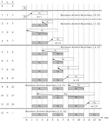
Now that we have seen how to streamline our dynamic-programming solution, and how to treat it as a top-down method, we are ready to see an algorithm that works in a purely greedy, top-down fashion. We give a straightforward, recursive solution as the procedure RECURSIVE-ACTIVITY-SELECTOR. It takes the start and finish times of the activities, represented as arrays s and f, as well as the starting indices i and j of the subproblem S_i.j it is to solve. It returns a maximum-size set of mutually compatible activities in S_i.j. We assume that the n input activities are ordered by monotonically increasing finish time, according to equation (16.1). If not, we can sort them into this order in O(n lg n) time, breaking ties arbitrarily. The initial call is RECURSIVE-ACTIVITY-SELECTOR(s, f, 0, n + 1).

RECURSIVE-ACTIVITY-SELECTOR(s, f, i, j)
1 m ← i + 1
2 while m  < j and sm < fi ▹ Find the first activity in Sij.
3     do m ← m + 1
4 if m < j
5    then return {am} ∪ RECURSIVE-ACTIVITY-SELECTOR(s, f, m, j)
6    else return Ø

Figure 16.1 shows the operation of the algorithm. In a given recursive call RECURSIVE-ACTIVITY-SELECTOR(s, f, i, j), the while loop of lines 2-3 looks for the first activity in S_ij. The loop examines a_i+1, a_i+2, ..., a_j-1, until it finds the first activity a_m that is compatible with a_i; such an activity has s_m ≥ f_i. If the loop terminates because it finds such an activity, the procedure returns in line 5 the union of {a_m} and the maximum-size subset of S_mj returned by the recursive call RECURSIVE-ACTIVITY-SELECTOR(s, f, m, j). Alternatively, the loop may terminate because m ≥ j, in which case we have examined all activities whose finish times are before that of a_j without finding one that is compatible with a_i. In this case, S_ij = Ø, and so the procedure returns Ø in line 6.

Figure 16.1: The operation of RECURSIVE-ACTIVITY-SELECTOR on the 11 activities given earlier. Activities considered in each recursive call appear between horizontal lines. The fictitious activity a₀ finishes at time 0, and in the initial call, RECURSIVE-ACTIVITY-SELECTOR(s, f, 0, 12), activity a₁ is selected. In each recursive call, the activities that have already been selected are shaded, and the activity shown in white is being considered. If the starting time of an activity occurs before the finish time of the most recently added activity (the arrow between them points left), it is rejected. Otherwise (the arrow points directly up or to the right), it is selected. The last recursive call, RECURSIVE-ACTIVITY-SELECTOR(s, f, 11, 12), returns Ø. The resulting set of selected activities is {a₁, a₄, a₈, a₁₁}.

Assuming that the activities have already been sorted by finish times, the running time of the call RECURSIVE-ACTIVITY-SELECTOR(s, f, 0, n + 1) is Θ(n), which we can see as follows. Over all recursive calls, each activity is examined exactly once in the while loop test of line 2. In particular, activity ak is examined in the last call made in which i < k.

An iterative greedy algorithm

We easily can convert our recursive procedure to an iterative one. The procedure RECURSIVE-ACTIVITY-SELECTOR is almost "tail recursive" (see Problem 7-4): it ends with a recursive call to itself followed by a union operation. It is usually a straightforward task to transform a tail-recursive procedure to an iterative form; in fact, some compilers for certain programming languages perform this task automatically. As written, RECURSIVE-ACTIVITY-SELECTOR works for any subproblem S_ij, but we have seen that we need to consider only subproblems for which j = n + 1, i.e., subproblems that consist of the last activities to finish.

The procedure GREEDY-ACTIVITY-SELECTOR is an iterative version of the procedure RECURSIVE-ACTIVITY-SELECTOR. It also assumes that the input activities are ordered by monotonically increasing finish time. It collects selected activities into a set A and returns this set when it is done.

GREEDY-ACTIVITY-SELECTOR(s, f)
1 n ← length[s]
2 A ← {a1}
3 i ← 1
4 for m ← 2 to n
5      do if sm ≥ fi
6            then A ← A ∪ {am}
7                 i ← m
8 return A

The procedure works as follows. The variable i indexes the most recent addition to A, corresponding to the activity a_i in the recursive version. Since the activities are considered in order of monotonically increasing finish time, f_i is always the maximum finish time of any activity in A. That is,

(16.4)

Lines 2-3 select activity a₁, initialize A to contain just this activity, and initialize i to index this activity. The for loop of lines 4-7 finds the earliest activity to finish in S_i.n+1. The loop considers each activity a_m in turn and adds a_m to A if it is compatible with all previously selected activities; such an activity is the earliest to finish in S_i.n+1. To see if activity a_m is compatible with every activity currently in A, it suffices by equation (16.4) to check (line 5) that its start time s_m is not earlier than the finish time f_i of the activity most recently added to A. If activity a_m is compatible, then lines 6-7 add activity a_m to A and set i to m. The set A returned by the call GREEDY-ACTIVITY-SELECTOR(s, f) is precisely the set returned by the call RECURSIVE-ACTIVITY-SELECTOR(s, f, 0, n + 1).

Like the recursive version, GREEDY-ACTIVITY-SELECTOR schedules a set of n activities in Θ(n) time, assuming that the activities were already sorted initially by their finish times.

Exercises 16.1-1

Give a dynamic-programming algorithm for the activity-selection problem, based on the recurrence (16.3). Have your algorithm compute the sizes c[i, j] as defined above and also produce the maximum-size subset A of activities. Assume that the inputs have been sorted as in equation (16.1). Compare the running time of your solution to the running time of GREEDY-ACTIVITY-SELECTOR.

Exercises 16.1-2

Suppose that instead of always selecting the first activity to finish, we instead select the last activity to start that is compatible with all previously selected activities. Describe how this approach is a greedy algorithm, and prove that it yields an optimal solution.

Exercises 16.1-3

Suppose that we have a set of activities to schedule among a large number of lecture halls. We wish to schedule all the activities using as few lecture halls as possible. Give an efficient greedy algorithm to determine which activity should use which lecture hall.

(This is also known as the interval-graph coloring problem. We can create an interval graph whose vertices are the given activities and whose edges connect incompatible activities. The smallest number of colors required to color every vertex so that no two adjacent vertices are given the same color corresponds to finding the fewest lecture halls needed to schedule all of the given activities.)

Exercises 16.1-4

Not just any greedy approach to the activity-selection problem produces a maximum-size set of mutually compatible activities. Give an example to show that the approach of selecting the activity of least duration from those that are compatible with previously selected activities does not work. Do the same for the approaches of always selecting the compatible activity that overlaps the fewest other remaining activities and always selecting the compatible remaining activity with the earliest start time.