|
|
< Day Day Up > |
|
Section 7.2 gave some intuition for the worst-case behavior of quicksort and for why we expect it to run quickly. In this section, we analyze the behavior of quicksort more rigorously. We begin with a worst-case analysis, which applies to either QUICKSORT or RANDOMIZED-QUICKSORT, and conclude with an average-case analysis of RANDOMIZED-QUICKSORT.
We saw in Section 7.2 that a worst-case split at every level of recursion in quicksort produces a Θ(n2) running time, which, intuitively, is the worst-case running time of the algorithm. We now prove this assertion.
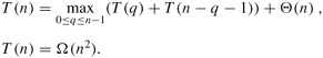
Using the substitution method (see Section 4.1), we can show that the running time of quicksort is O(n2). Let T (n) be the worst-case time for the procedure QUICKSORT on an input of size n. We have the recurrence
where the parameter q ranges from 0 to n - 1 because the procedure PARTITION produces two subproblems with total size n - 1. We guess that T (n) ≤ cn2 for some constant c. Substituting this guess into recurrence (7.1), we obtain
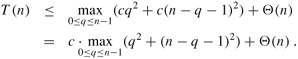
The expression q2 +(n-q-1)2 achieves a maximum over the parameter's range 0 ≤ q ≤ n - 1 at either endpoint, as can be seen since the second derivative of the expression with respect to q is positive (see Exercise 7.4-3). This observation gives us the bound max≤q≤n-1(q2+ (n - q - 1)2) ≤ (n - 1)2 = n2 - 2n + 1. Continuing with our bounding of T (n), we obtain
|
T(n) |
≤ |
cn2 - c(2n - 1) + Θ(n) |
|
≤ |
cn2, |
since we can pick the constant c large enough so that the c(2n - 1) term dominates the Θ(n) term. Thus, T (n) = O(n2). We saw in Section 7.2 a specific case in which quicksort takes Θ(n2) time: when partitioning is unbalanced. Alternatively, Exercise 7.4-1 asks you to show that recurrence (7.1) has a solution of T (n) = Θ(n2). Thus, the (worst-case) running time of quicksort is Θ(n2).
We have already given an intuitive argument why the average-case running time of RANDOMIZED-QUICKSORT is O(n lg n): if, in each level of recursion, the split induced by RANDOMIZED-PARTITION puts any constant fraction of the elements on one side of the partition, then the recursion tree has depth Θ(lg n), and O(n) work is performed at each level. Even if we add new levels with the most unbalanced split possible between these levels, the total time remains O(n lg n). We can analyze the expected running time of RANDOMIZED-QUICKSORT precisely by first understanding how the partitioning procedure operates and then using this understanding to derive an O(n lg n) bound on the expected running time. This upper bound on the expected running time, combined with the Θ(n lg n) best-case bound we saw in Section 7.2, yields a Θ(n lg n) expected running time.
The running time of QUICKSORT is dominated by the time spent in the PARTITION procedure. Each time the PARTITION procedure is called, a pivot element is selected, and this element is never included in any future recursive calls to QUICK-SORT and PARTITION. Thus, there can be at most n calls to PARTITION over the entire execution of the quicksort algorithm. One call to PARTITION takes O(1) time plus an amount of time that is proportional to the number of iterations of the for loop in lines 3-6. Each iteration of this for loop performs a comparison inline 4, comparing the pivot element to another element of the array A. Therefore, if we can count the total number of times that line 4 is executed, we can bound the total time spent in the for loop during the entire execution of QUICKSORT.
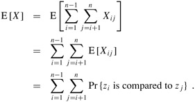
Let X be the number of comparisons performed in line 4 of PARTITION over the entire execution of QUICKSORT on an n-element array. Then the running time of QUICKSORT is O(n + X).
Proof By the discussion above, there are n calls to PARTITION, each of which does a constant amount of work and then executes the for loop some number of times. Each iteration of the for loop executes line 4.
Our goal, therefore is to compute X, the total number of comparisons performed in all calls to PARTITION. We will not attempt to analyze how many comparisons are made in each call to PARTITION. Rather, we will derive an overall bound on the total number of comparisons. To do so, we must understand when the algorithm compares two elements of the array and when it does not. For ease of analysis, we rename the elements of the array A as z1, z2,..., zn, with zi being the ith smallest element. We also define the set Zij = {zi, zi+1,..., zj} to be the set of elements between zi and zj, inclusive.
When does the algorithm compare zi and zj? To answer this question, we first observe that each pair of elements is compared at most once. Why? Elements are compared only to the pivot element and, after a particular call of PARTITION finishes, the pivot element used in that call is never again compared to any other elements.
Our analysis uses indicator random variables (see Section 5.2). We define
Xij = I {zi is compared to zj} ,
where we are considering whether the comparison takes place at any time during the execution of the algorithm, not just during one iteration or one call of PARTITION. Since each pair is compared at most once, we can easily characterize the total number of comparisons performed by the algorithm:
Taking expectations of both sides, and then using linearity of expectation and Lemma 5.1, we obtain
It remains to compute Pr {zi is compared to zj}.
It is useful to think about when two items are not compared. Consider an input to quicksort of the numbers 1 through 10 (in any order), and assume that the first pivot element is 7. Then the first call to PARTITION separates the numbers into two sets: {1, 2, 3, 4, 5, 6} and {8, 9, 10}. In doing so, the pivot element 7 is compared to all other elements, but no number from the first set (e.g., 2) is or ever will be compared to any number from the second set (e.g., 9).
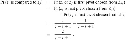
In general, once a pivot x is chosen with zi < x < zj, we know that zi and zj cannot be compared at any subsequent time. If, on the other hand, zi is chosen as a pivot before any other item in Zij, then zi will be compared to each item in Zij, except for itself. Similarly, if zj is chosen as a pivot before any other item in Zij, then zj will be compared to each item in Zij , except for itself. In our example, the values 7 and 9 are compared because 7 is the first item from Z7,9 to be chosen as a pivot. In contrast, 2 and 9 will never be compared because the first pivot element chosen from Z2,9 is 7. Thus, zi and zj are compared if and only if the first element to be chosen as a pivot from Zij is either zi or zj.
We now compute the probability that this event occurs. Prior to the point at which an element from Zij has been chosen as a pivot, the whole set Zij is together in the same partition. Therefore, any element of Zij is equally likely to be the first one chosen as a pivot. Because the set Zij has j - i + 1 elements, the probability that any given element is the first one chosen as a pivot is 1/(j - i + 1). Thus, we have
The second line follows because the two events are mutually exclusive. Combining equations (7.2) and (7.3), we get that
We can evaluate this sum using a change of variables (k = j - i) and the bound on the harmonic series in equation (A.7):
| (7.4) | 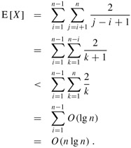 |
Thus we conclude that, using RANDOMIZED-PARTITION, the expected running time of quicksort is O(n lg n).
Show that q2 + (n - q - 1)2 achieves a maximum over q = 0, 1,..., n - 1 when q = 0 or q = n - 1.
The running time of quicksort can be improved in practice by taking advantage of the fast running time of insertion sort when its input is "nearly" sorted. When quicksort is called on a subarray with fewer than k elements, let it simply return without sorting the subarray. After the top-level call to quicksort returns, run insertion sort on the entire array to finish the sorting process. Argue that this sorting algorithm runs in O(nk + n lg(n/k)) expected time. How should k be picked, both in theory and in practice?
Consider modifying the PARTITION procedure by randomly picking three elements from array A and partitioning about their median (the middle value of the three elements). Approximate the probability of getting at worst an αto-(1 - α) split, as a function of α in the range 0 < α < 1.
The version of PARTITION given in this chapter is not the original partitioning algorithm. Here is the original partition algorithm, which is due to T. Hoare:
HOARE-PARTITION(A, p, r)
 1  x ← A[p]
 2  i ← p - 1
 3  j ← r + 1
 4  while TRUE
 5      do repeat j ← j - 1
 6           until A[j] ≤ x
 7         repeat i ← i + 1
 8           until A[i] ≥ x
 9         if i < j
10            then exchange A[i] ↔ A[j]
11            else return j
Demonstrate the operation of HOARE-PARTITION on the array A = 〈13, 19, 9, 5, 12, 8, 7, 4, 11, 2, 6, 21〉, showing the values of the array and auxiliary values after each iteration of the for loop in lines 4-11.
The next three questions ask you to give a careful argument that the procedure HOARE-PARTITION is correct. Prove the following:
The indices i and j are such that we never access an element of A outside the subarray A[p ‥ r].
When HOARE-PARTITION terminates, it returns a value j such that p ≤ j < r.
Every element of A[p ‥ j] is less than or equal to every element of A[j +1 ‥ r] when HOARE-PARTITION terminates.
The PARTITION procedure in Section 7.1 separates the pivot value (originally in A[r]) from the two partitions it forms. The HOARE-PARTITION procedure, on the other hand, always places the pivot value (originally in A[p]) into one of the two partitions A[p ‥ j] and A[j + 1 ‥ r]. Since p ≤ j < r, this split is always nontrivial.
Rewrite the QUICKSORT procedure to use HOARE-PARTITION.
An alternative analysis of the running time of randomized quicksort focuses on the expected running time of each individual recursive call to QUICKSORT, rather than on the number of comparisons performed.
Argue that, given an array of size n, the probability that any particular element is chosen as the pivot is 1/n. Use this to define indicator random variables Xi = I{ith smallest element is chosen as the pivot}. What is E [Xi]?
Let T (n) be a random variable denoting the running time of quicksort on an array of size n. Argue that
Show that equation (7.5) simplifies to
Show that
(Hint: Split the summation into two parts, one for k = 1, 2,..., ⌈n/2⌉ - 1 and one for k = ⌈n/2⌉,..., n - 1.)
Using the bound from equation (7.7), show that the recurrence in equation (7.6) has the solution E [T (n)] = Θ(n lg n). (Hint: Show, by substitution, that E[T (n)] ≤ an log n - bn for some positive constants a and b.)
Professors Howard, Fine, and Howard have proposed the following "elegant" sorting algorithm:
STOOGE-SORT(A, i, j)
1  if A[i] > A[j]
2     then exchange A[i] ↔ A[j]
3  if i + 1 ≥ j
4     then return
5  k ← ⌊(j - i + 1)/3⌋             ▹ Round down.
6  STOOGE-SORT(A, i, j - k)         ▹ First two-thirds.
7  STOOGE-SORT(A, i + k, j)         ▹ Last two-thirds.
8  STOOGE-SORT(A, i, j - k)         ▹ First two-thirds again.
Argue that, if n = length[A], then STOOGE-SORT(A, 1, length[A]) correctly sorts the input array A[1 ‥ n].
Give a recurrence for the worst-case running time of STOOGE-SORT and a tight asymptotic (Θ-notation) bound on the worst-case running time.
Compare the worst-case running time of STOOGE-SORT with that of insertion sort, merge sort, heapsort, and quicksort. Do the professors deserve tenure?
The QUICKSORT algorithm of Section 7.1 contains two recursive calls to itself. After the call to PARTITION, the left subarray is recursively sorted and then the right subarray is recursively sorted. The second recursive call in QUICKSORT is not really necessary; it can be avoided by using an iterative control structure. This technique, called tail recursion, is provided automatically by good compilers. Consider the following version of quicksort, which simulates tail recursion.
QUICKSORT'(A, p, r)
1  while p < r
2        do ▸ Partition and sort left subarray.
3             q ← PARTITION(A, p, r)
4             QUICKSORT'(A, p, q - 1)
5             p ← q + 1
Argue that QUICKSORT'(A, 1, length[A]) correctly sorts the array A.
Compilers usually execute recursive procedures by using a stack that contains pertinent information, including the parameter values, for each recursive call. The information for the most recent call is at the top of the stack, and the information for the initial call is at the bottom. When a procedure is invoked, its information is pushed onto the stack; when it terminates, its information is popped. Since we assume that array parameters are represented by pointers, the information for each procedure call on the stack requires O(1) stack space. The stack depth is the maximum amount of stack space used at any time during a computation.
Describe a scenario in which the stack depth of QUICKSORT' is Θ(n) on an n-element input array.
Modify the code for QUICKSORT' so that the worst-case stack depth is Θ(lg n). Maintain the O(n lg n) expected running time of the algorithm.
One way to improve the RANDOMIZED-QUICKSORT procedure is to partition around a pivot that is chosen more carefully than by picking a random element from the subarray. One common approach is the median-of-3 method: choose the pivot as the median (middle element) of a set of 3 elements randomly selected from the subarray. (See Exercise 7.4-6.) For this problem, let us assume that the elements in the input array A[1 ‥ n] are distinct and that n ≥ 3. We denote the sorted output array by A'[1 ‥ n]. Using the median-of-3 method to choose the pivot element x, define pi = Pr{x = A'[i]}.
Give an exact formula for pi as a function of n and i for i = 2, 3,..., n - 1. (Note that p1 = pn = 0.)
By what amount have we increased the likelihood of choosing the pivot as x = A'[⌊(n + 1/2⌋], the median of A[1 ‥ n], compared to the ordinary implementation? Assume that n → ∞, and give the limiting ratio of these probabilities.
If we define a "good" split to mean choosing the pivot as x = A'[i], where n/ ≤ i ≤ 2n/3, by what amount have we increased the likelihood of getting a good split compared to the ordinary implementation? (Hint: Approximate the sum by an integral.)
Argue that in the Ω(n lg n) running time of quicksort, the median-of-3 method affects only the constant factor.
Consider a sorting problem in which the numbers are not known exactly. Instead, for each number, we know an interval on the real line to which it belongs. That is, we are given n closed intervals of the form [ai, bi], where ai ≤ bi. The goal is to fuzzy-sort these intervals, i.e., produce a permutation 〈i1, i2,..., in〉 of the intervals such that there exist ![]() , satisfying c1 ≤ c2 ≤ ··· ≤ cn.
, satisfying c1 ≤ c2 ≤ ··· ≤ cn.
Design an algorithm for fuzzy-sorting n intervals. Your algorithm should have the general structure of an algorithm that quicksorts the left endpoints (the ai 's), but it should take advantage of overlapping intervals to improve the running time. (As the intervals overlap more and more, the problem of fuzzy-sorting the intervals gets easier and easier. Your algorithm should take advantage of such overlapping, to the extent that it exists.)
Argue that your algorithm runs in expected time Θ(n lg n) in general, but runs in expected time Θ(n) when all of the intervals overlap (i.e., when there exists a value x such that x ∈ [ai, bi] for all i). Your algorithm should not be checking for this case explicitly; rather, its performance should naturally improve as the amount of overlap increases.
|
|
< Day Day Up > |
|