|
|
< Day Day Up > |
|
Like a binomial heap, a Fibonacci heap is a collection of min-heap-ordered trees. The trees in a Fibonacci heap are not constrained to be binomial trees, however. Figure 20.1(a) shows an example of a Fibonacci heap.
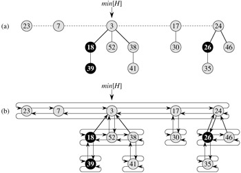
Unlike trees within binomial heaps, which are ordered, trees within Fibonacci heaps are rooted but unordered. As Figure 20.1(b) shows, each node x contains a pointer p[x] to its parent and a pointer child[x] to any one of its children. The children of x are linked together in a circular, doubly linked list, which we call the child list of x. Each child y in a child list has pointers left[y] and right[y] that point to y's left and right siblings, respectively. If node y is an only child, then left[y] = right[y] = y. The order in which siblings appear in a child list is arbitrary.
Circular, doubly linked lists (see Section 10.2) have two advantages for use in Fibonacci heaps. First, we can remove a node from a circular, doubly linked list in O(1) time. Second, given two such lists, we can concatenate them (or "splice" them together) into one circular, doubly linked list in O(1) time. In the descriptions of Fibonacci heap operations, we shall refer to these operations informally, letting the reader fill in the details of their implementations.
Two other fields in each node will be of use. The number of children in the child list of node x is stored in degree[x]. The boolean-valued field mark[x] indicates whether node x has lost a child since the last time x was made the child of another node. Newly created nodes are unmarked, and a node x becomes unmarked whenever it is made the child of another node. Until we look at the DECREASE-KEY operation in Section 20.3, we will just set all mark fields to FALSE.
A given Fibonacci heap H is accessed by a pointer min[H] to the root of a tree containing a minimum key; this node is called the minimum node of the Fibonacci heap. If a Fibonacci heap H is empty, then min[H] = NIL.
The roots of all the trees in a Fibonacci heap are linked together using their left and right pointers into a circular, doubly linked list called the root list of the Fibonacci heap. The pointer min[H] thus points to the node in the root list whose key is minimum. The order of the trees within a root list is arbitrary.
We rely on one other attribute for a Fibonacci heap H: the number of nodes currently in H is kept in n[H].
As mentioned, we shall use the potential method of Section 17.3 to analyze the performance of Fibonacci heap operations. For a given Fibonacci heap H, we indicate by t(H) the number of trees in the root list of H and by m(H) the number of marked nodes in H. The potential of Fibonacci heap H is then defined by
(We will gain some intuition for this potential function in Section 20.3.) For example, the potential of the Fibonacci heap shown in Figure 20.1 is 5 + 2·3 = 11. The potential of a set of Fibonacci heaps is the sum of the potentials of its constituent Fibonacci heaps. We shall assume that a unit of potential can pay for a constant amount of work, where the constant is sufficiently large to cover the cost of any of the specific constant-time pieces of work that we might encounter.
We assume that a Fibonacci heap application begins with no heaps. The initial potential, therefore, is 0, and by equation (20.1), the potential is nonnegative at all subsequent times. From equation (17.3), an upper bound on the total amortized cost is thus an upper bound on the total actual cost for the sequence of operations.
The amortized analyses we shall perform in the remaining sections of this chapter assume that there is a known upper bound D(n) on the maximum degree of any node in an n-node Fibonacci heap. Exercise 20.2-3 shows that when only the mergeable-heap operations are supported, D(n) ≤ ⌊lg n⌋. In Section 20.3, we shall show that when we support DECREASE-KEY and DELETE as well, D(n) = O(lg n).
|
|
< Day Day Up > |
|