Worst-case partitioning

The worst-case behavior for quicksort occurs when the partitioning routine produces one subproblem with n - 1 elements and one with 0 elements. (This claim is proved in Section 7.4.1.) Let us assume that this unbalanced partitioning arises in each recursive call. The partitioning costs Θ(n) time. Since the recursive call on an array of size 0 just returns, T(0) = Θ(1), and the recurrence for the running time is

Intuitively, if we sum the costs incurred at each level of the recursion, we get an arithmetic series (equation (A.2)), which evaluates to Θ(n²). Indeed, it is straightforward to use the substitution method to prove that the recurrence T(n) = T(n - 1) + Θ(n) has the solution T(n) = Θ(n²). (See Exercise 7.2-1.)

Thus, if the partitioning is maximally unbalanced at every recursive level of the algorithm, the running time is Θ(n²). Therefore the worst-case running time of quicksort is no better than that of insertion sort. Moreover, the Θ(n²) running time occurs when the input array is already completely sorted-a common situation in which insertion sort runs in O(n) time.

Best-case partitioning

In the most even possible split, PARTITION produces two subproblems, each of size no more than n/2, since one is of size ⌊n/2⌋ and one of size ⌈n/2⌉- 1. In this case, quicksort runs much faster. The recurrence for the running time is then

T (n) ≤ 2T (n/2) + Θ(n) ,

which by case 2 of the master theorem (Theorem 4.1) has the solution T (n) = O(n lg n). Thus, the equal balancing of the two sides of the partition at every level of the recursion produces an asymptotically faster algorithm.

Balanced partitioning

The average-case running time of quicksort is much closer to the best case than to the worst case, as the analyses in Section 7.4 will show. The key to understanding why is to understand how the balance of the partitioning is reflected in the recurrence that describes the running time.

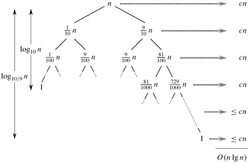
Suppose, for example, that the partitioning algorithm always produces a 9-to-1 proportional split, which at first blush seems quite unbalanced. We then obtain the recurrence

T(n) ≤ T (9n/10) + T (n/10) + cn

on the running time of quicksort, where we have explicitly included the constant c hidden in the Θ(n) term. Figure 7.4 shows the recursion tree for this recurrence. Notice that every level of the tree has cost cn, until a boundary condition is reached at depth log₁₀n = Θ(lgn), and then the levels have cost at most cn. The recursion terminates at depth log_10/9n = Θ(lg n). The total cost of quicksort is therefore O(n lg n). Thus, with a 9-to-1 proportional split at every level of recursion, which intuitively seems quite unbalanced, quicksort runs in O(n lg n) time-asymptotically the same as if the split were right down the middle. In fact, even a 99-to-1 split yields an O(n lg n) running time. The reason is that any split of constant proportionality yields a recursion tree of depth Θ(lg n), where the cost at each level is O(n). The running time is therefore O(n lg n) whenever the split has constant proportionality.

Intuition for the average case

To develop a clear notion of the average case for quicksort, we must make an assumption about how frequently we expect to encounter the various inputs. The behavior of quicksort is determined by the relative ordering of the values in the array elements given as the input, and not by the particular values in the array. As in our probabilistic analysis of the hiring problem in Section 5.2, we will assume for now that all permutations of the input numbers are equally likely.

When we run quicksort on a random input array, it is unlikely that the partitioning always happens in the same way at every level, as our informal analysis has assumed. We expect that some of the splits will be reasonably well balanced and that some will be fairly unbalanced. For example, Exercise 7.2-6 asks you to show that about 80 percent of the time PARTITION produces a split that is more balanced than 9 to 1, and about 20 percent of the time it produces a split that is less balanced than 9 to 1.

In the average case, PARTITION produces a mix of "good" and "bad" splits. In a recursion tree for an average-case execution of PARTITION, the good and bad splits are distributed randomly throughout the tree. Suppose for the sake of intuition, however, that the good and bad splits alternate levels in the tree, and that the good splits are best-case splits and the bad splits are worst-case splits. Figure 7.5(a) shows the splits at two consecutive levels in the recursion tree. At the root of the tree, the cost is n for partitioning, and the subarrays produced have sizes n - 1 and 0: the worst case. At the next level, the subarray of size n - 1 is best-case partitioned into subarrays of size (n - 1)/2 - 1 and (n - 1)/2. Let's assume that the boundary-condition cost is 1 for the subarray of size 0.

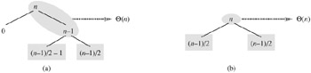
The combination of the bad split followed by the good split produces three subarrays of sizes 0, (n - 1)/2 - 1, and (n - 1)/2 at a combined partitioning cost of Θ(n) + Θ(n - 1) = Θ(n). Certainly, this situation is no worse than that in Figure 7.5(b), namely a single level of partitioning that produces two subarrays of size (n - 1)/2, at a cost of Θ(n). Yet this latter situation is balanced! Intuitively, the Θ(n - 1) cost of the bad split can be absorbed into the Θ(n) cost of the good split, and the resulting split is good. Thus, the running time of quicksort, when levels alternate between good and bad splits, is like the running time for good splits alone: still O(n lg n), but with a slightly larger constant hidden by the O-notation. We shall give a rigorous analysis of the average case in Section 7.4.2.