|
|
< Day Day Up > |
|
In biological applications, we often want to compare the DNA of two (or more) different organisms. A strand of DNA consists of a string of molecules called bases, where the possible bases are adenine, guanine, cytosine, and thymine. Representing each of these bases by their initial letters, a strand of DNA can be expressed as a string over the finite set {A, C, G, T}. (See Appendix C for a definition of a string.) For example, the DNA of one organism may be S1= ACCGGTCGAGTGCGCGGAAGCCGGCCGAA, while the DNA of another organism may be S2 = GTCGTTCGGAATGCCGTTGCTCTGTAAA. One goal of comparing two strands of DNA is to determine how "similar" the two strands are, as some measure of how closely related the two organisms are. Similarity can be and is defined in many different ways. For example, we can say that two DNA strands are similar if one is a substring of the other. (Chapter 32 explores algorithms to solve this problem.) In our example, neither S1 nor S2 is a substring of the other. Alternatively, we could say that two strands are similar if the number of changes needed to turn one into the other is small. (Problem 15-3 looks at this notion.) Yet another way to measure the similarity of strands S1 and S2 is by finding a third strand S3 in which the bases in S3 appear in each of S1 and S2; these bases must appear in the same order, but not necessarily consecutively. The longer the strand S3 we can find, the more similar S1 and S2 are. In our example, the longest strand S3 is GTCGTCGGAAGCCGGCCGAA.
We formalize this last notion of similarity as the longest-common-subsequence problem. A subsequence of a given sequence is just the given sequence with zero or more elements left out. Formally, given a sequence X = 〈x1, x2, ..., xm〉, another sequence Z = 〈z1, z2, ..., zk〉 is a subsequence of X if there exists a strictly increasing sequence 〈i1,i2, ..., ik〉 of indices of X such that for all j = 1, 2, ..., k, we have xij = zj . For example, Z = 〈B, C, D, B〉 is a subsequence of X = 〈A, B, C, B, D, A, B〉 with corresponding index sequence 〈2, 3, 5, 7〉.
Given two sequences X and Y , we say that a sequence Z is a common subsequence of X and Y if Z is a subsequence of both X and Y . For example, if X = 〈A, B, C, B, D, A, B〉 and Y = 〈B, D, C, A, B, A〉, the sequence 〈B, C, A〉 is a common subsequence of both X and Y . The sequence 〈B, C, A〉 is not a longest common subsequence (LCS) of X and Y , however, since it has length 3 and the sequence 〈B, C, B, A〉, which is also common to both X and Y , has length 4. The sequence 〈B, C, B, A〉 is an LCS of X and Y , as is the sequence 〈B, D, A, B〉, since there is no common subsequence of length 5 or greater.
In the longest-common-subsequence problem, we are given two sequences X = 〈x1, x2, ..., xm〉 and Y = 〈y1, y2, ..., yn〉 and wish to find a maximum-length common subsequence of X and Y . This section shows that the LCS problem can be solved efficiently using dynamic programming.
A brute-force approach to solving the LCS problem is to enumerate all subsequences of X and check each subsequence to see if it is also a subsequence of Y , keeping track of the longest subsequence found. Each subsequence of X corresponds to a subset of the indices {1, 2, ..., m} of X. There are 2m subsequences of X, so this approach requires exponential time, making it impractical for long sequences.
The LCS problem has an optimal-substructure property, however, as the following theorem shows. As we shall see, the natural classes of subproblems correspond to pairs of "prefixes" of the two input sequences. To be precise, given a sequence X = 〈x1, x2, ..., xm〉, we define the ith prefix of X, for i = 0, 1, ..., m, as Xi = 〈x1, x2, ..., xi〉. For example, if X = 〈A, B, C, B, D, A, B〉, then X4 = 〈A, B, C, B〉 and X0 is the empty sequence.
Let X = 〈x1, x2, ..., xm〉 and Y = 〈y1, y2, ..., yn〉 be sequences, and let Z = 〈z1, z2, ..., zk〉 be any LCS of X and Y.
If xm = yn, then zk = xm = yn and Zk-1 is an LCS of Xm-1 and Yn-1.
If xm ≠ yn, then zk ≠ xm implies that Z is an LCS of Xm-1 and Y.
If xm ≠ yn, then zk ≠ yn implies that Z is an LCS of X and Yn-1.
Proof (1) If zk ≠ xm, then we could append xm = yn to Z to obtain a common subsequence of X and Y of length k + 1, contradicting the supposition that Z is a longest common subsequence of X and Y . Thus, we must have zk = xm = yn. Now, the prefix Zk-1 is a length-(k - 1) common subsequence of Xm-1 and Yn-1. We wish to show that it is an LCS. Suppose for the purpose of contradiction that there is a common subsequence W of Xm-1 and Yn-1 with length greater than k - 1. Then, appending xm = yn to W produces a common subsequence of X and Y whose length is greater than k, which is a contradiction.
(2) If zk ≠ xm, then Z is a common subsequence of Xm-1 and Y. If there were a common subsequence W of Xm-1 and Y with length greater than k, then W would also be a common subsequence of Xm and Y , contradicting the assumption that Z is an LCS of X and Y.
(3) The proof is symmetric to (2).
The characterization of Theorem 15.1 shows that an LCS of two sequences contains within it an LCS of prefixes of the two sequences. Thus, the LCS problem has an optimal-substructure property. A recursive solution also has the overlapping-subproblems property, as we shall see in a moment.
Theorem 15.1 implies that there are either one or two subproblems to examine when finding an LCS of X = 〈x1, x2, ..., xm〉 and Y = 〈y1, y2, ..., yn〉. If xm = yn, we must find an LCS of Xm-1 and Yn-1. Appending xm = yn to this LCS yields an LCS of X and Y. If xm ≠ yn, then we must solve two subproblems: finding an LCS of Xm-1 and Y and finding an LCS of X and Yn-1. Whichever of these two LCS's is longer is an LCS of X and Y. Because these cases exhaust all possibilities, we know that one of the optimal subproblem solutions must be used within an LCS of X and Y .
We can readily see the overlapping-subproblems property in the LCS problem. To find an LCS of X and Y , we may need to find the LCS's of X and Yn-1 and of Xm-1 and Y . But each of these subproblems has the subsubproblem of finding the LCS of Xm-1 and Yn-1. Many other subproblems share subsubproblems.
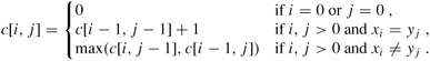
As in the matrix-chain multiplication problem, our recursive solution to the LCS problem involves establishing a recurrence for the value of an optimal solution. Let us define c[i, j] to be the length of an LCS of the sequences Xi and Yj . If either i = 0 or j = 0, one of the sequences has length 0, so the LCS has length 0. The optimal substructure of the LCS problem gives the recursive formula
Observe that in this recursive formulation, a condition in the problem restricts which subproblems we may consider. When xi = yj , we can and should consider the subproblem of finding the LCS of Xi-1 and Yj-1. Otherwise, we in stead consider the two subproblems of finding the LCS of Xi and Yj-1 and of Xi-1 and Yj. In the previous dynamic-programming algorithms we have examined-for assembly-line scheduling and matrix-chain multiplication-no subproblems were ruled out due to conditions in the problem. Finding the LCS is not the only dynamic-programming algorithm that rules out subproblems based on conditions in the problem. For example, the edit-distance problem (see Problem 15-3) has this characteristic.
Based on equation (15.14), we could easily write an exponential-time recursive algorithm to compute the length of an LCS of two sequences. Since there are only Θ(mn) distinct subproblems, however, we can use dynamic programming to compute the solutions bottom up.
Procedure LCS-LENGTH takes two sequences X = 〈x1, x2, ..., xm〉 and Y = 〈y1, y2, ..., yn〉 as inputs. It stores the c[i, j] values in a table c[0 ‥ m, 0 ‥ n] whose entries are computed in row-major order. (That is, the first row of c is filled in from left to right, then the second row, and so on.) It also maintains the table b[1 ‥ m, 1 ‥ n] to simplify construction of an optimal solution. Intuitively, b[i, j] points to the table entry corresponding to the optimal subproblem solution chosen when computing c[i, j]. The procedure returns the b and c tables; c[m, n] contains the length of an LCS of X and Y.
LCS-LENGTH(X, Y)
 1 m ← length[X]
 2 n ← length[Y]
 3 for i ← 1 to m
 4      do c[i, 0] ← 0
 5 for j ← 0 to n
 6      do c[0, j] ← 0
 7 for i ← 1 to m
 8      do for j ← 1 to n
 9             do if xi = yj
10                   then c[i, j] ← c[i - 1, j - 1] + 1
11                        b[i, j] ← "↖"
12                   else if c[i - 1, j] ≥ c[i, j - 1]
13                           then c[i, j] ← c[i - 1, j]
14                                b[i, j] ← "↑"
15                           else c[i, j] ← c[i, j - 1]
16                                b[i, j] ← ←
17 return c and b
Figure 15.6 shows the tables produced by LCS-LENGTH on the sequences X = 〈A, B, C, B, D, A, B〉 and Y = 〈B, D, C, A, B, A〉. The running time of the procedure is O(mn), since each table entry takes O(1) time to compute.
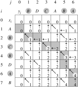
The b table returned by LCS-LENGTH can be used to quickly construct an LCS of X = 〈x1, x2, ..., xm〉 and Y = 〈y1, y2, ..., yn〉. We simply begin at b[m, n] and trace through the table following the arrows. Whenever we encounter a "↖" in entry b[i, j], it implies that xi = yj is an element of the LCS. The elements of the LCS are encountered in reverse order by this method. The following recursive procedure prints out an LCS of X and Y in the proper, forward order. The initial invocation is PRINT-LCS(b, X, length[X], length[Y]).
PRINT-LCS(b, X, i, j)
1 if i = 0 or j = 0
2     then return
3 if b[i, j] = "↖"
4     then PRINT-LCS(b, X, i - 1, j - 1)
5          print xi
6 elseif b[i, j] = "↑"
7    then PRINT-LCS(b, X, i - 1, j)
8 else PRINT-LCS(b, X, i, j - 1)
For the b table in Figure 15.6, this procedure prints "BCBA." The procedure takes time O(m + n), since at least one of i and j is decremented in each stage of the recursion.
Once you have developed an algorithm, you will often find that you can improve on the time or space it uses. This is especially true of straightforward dynamic-programming algorithms. Some changes can simplify the code and improve constant factors but otherwise yield no asymptotic improvement in performance. Others can yield substantial asymptotic savings in time and space.
For example, we can eliminate the b table altogether. Each c[i, j] entry depends on only three other c table entries: c[i - 1, j - 1], c[i - 1, j], and c[i, j - 1]. Given the value of c[i, j], we can determine in O(1) time which of these three values was used to compute c[i, j], without inspecting table b. Thus, we can reconstruct an LCS in O(m + n) time using a procedure similar to PRINT-LCS. (Exercise 15.4-2 asks you to give the pseudocode.) Although we save Θ(mn) space by this method, the auxiliary space requirement for computing an LCS does not asymptotically decrease, since we need Θ(mn) space for the c table anyway.
We can, however, reduce the asymptotic space requirements for LCS-LENGTH, since it needs only two rows of table c at a time: the row being computed and the previous row. (In fact, we can use only slightly more than the space for one row of c to compute the length of an LCS. See Exercise 15.4-4.) This improvement works if we need only the length of an LCS; if we need to reconstruct the elements of an LCS, the smaller table does not keep enough information to retrace our steps in O(m + n) time.
Show how to reconstruct an LCS from the completed c table and the original sequences X = 〈x1, x2, ..., xm〉 and Y = 〈y1, y2, ..., yn〉 in O(m +n) time, without using the b table.
Show how to compute the length of an LCS using only 2 · min(m, n) entries in the c table plus O(1) additional space. Then show how to do this using min(m, n) entries plus O(1) additional space.
Give an O(n2)-time algorithm to find the longest monotonically increasing subsequence of a sequence of n numbers.
Give an O(n lg n)-time algorithm to find the longest monotonically increasing sub-sequence of a sequence of n numbers. (Hint: Observe that the last element of a candidate subsequence of length i is at least as large as the last element of a candidate subsequence of length i - 1. Maintain candidate subsequences by linking them through the input sequence.)
|
|
< Day Day Up > |
|